
Thanks for following our blog. Our goal is to provide you with the most recent information about our business and landslide related issues and initiatives in Western North Carolina. So stay tuned in, especially when we get a lot of rain!.
A new look at a devastating landslide of the 1916 storm–the Jacks Branch debris flow
Reply
Note: This post is based on Jule Hubbard’s 2016 article, linked here. It’s a fascinating piece that does an excellent job capturing the human impacts of a notable landslide during the 1916 storm. You should give it a read before continuing…
Prior to Helene, landslide geologists in western North Carolina devoted considerable energy towards studying the dual hurricane event of 1916 and the effects of such a “superstorm” on mountain slopes. Useful landslide information from the 1916 storm was–and still is–hard to come by, with stories maintained in relatively local oral traditions often providing the most detailed (and elusive) accounts. Jule Hubbard of the Wilkes Journal-Patriot skillfully developed written and oral records of one 1916 debris flow landslide into a 2016 article, linked at the top of the post. Interestingly, this debris flow occurred on a stream called Jacks Branch in the Brushy Mountains, a smaller range southeast of the Blue Ridge Escarpment and the higher peaks to its northwest.
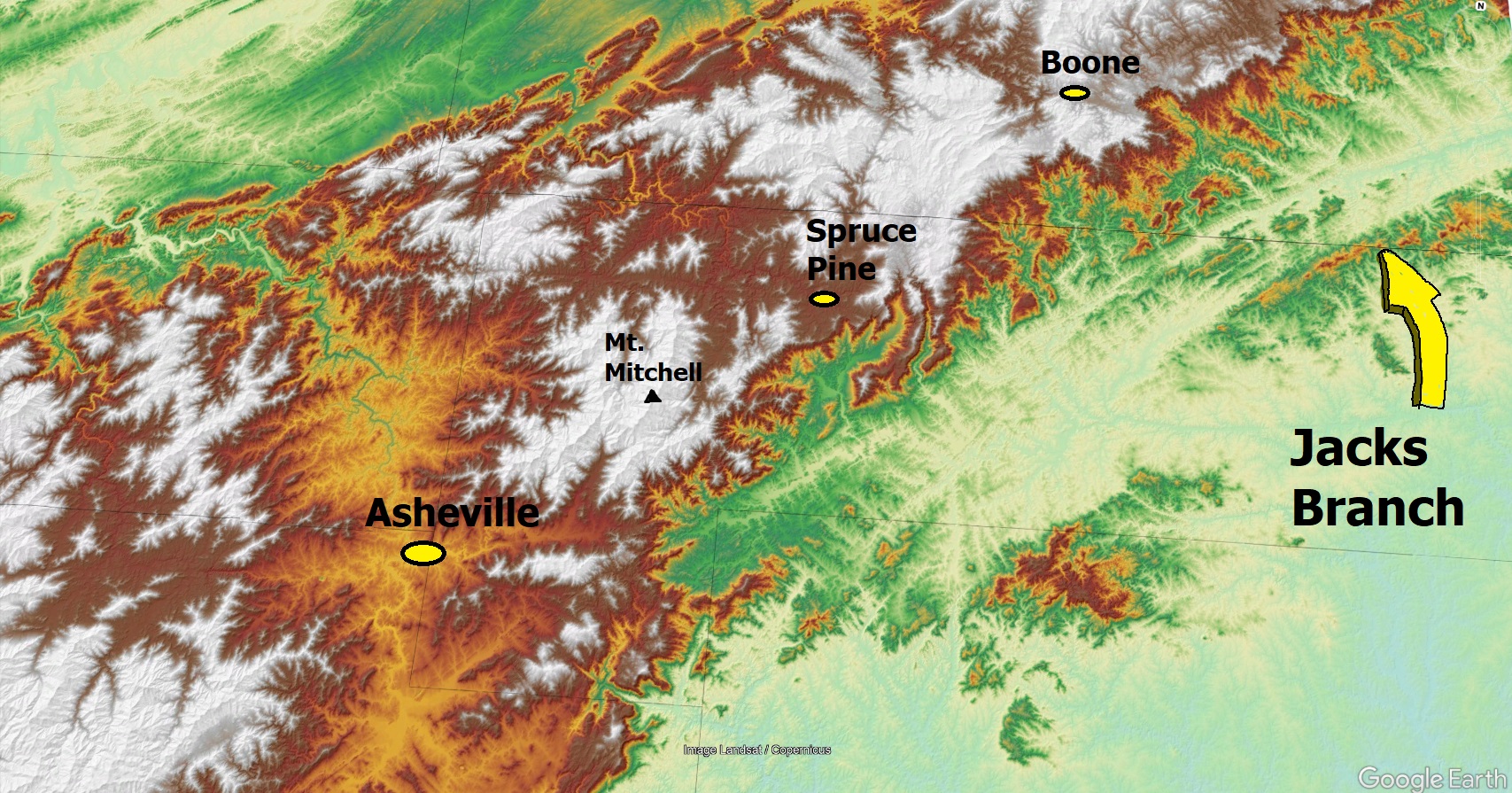
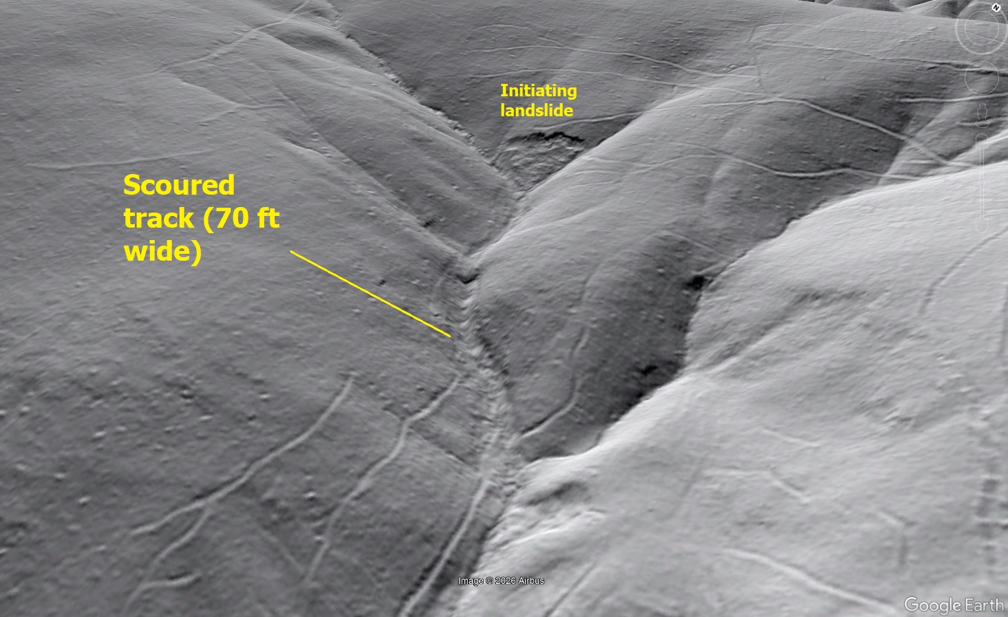
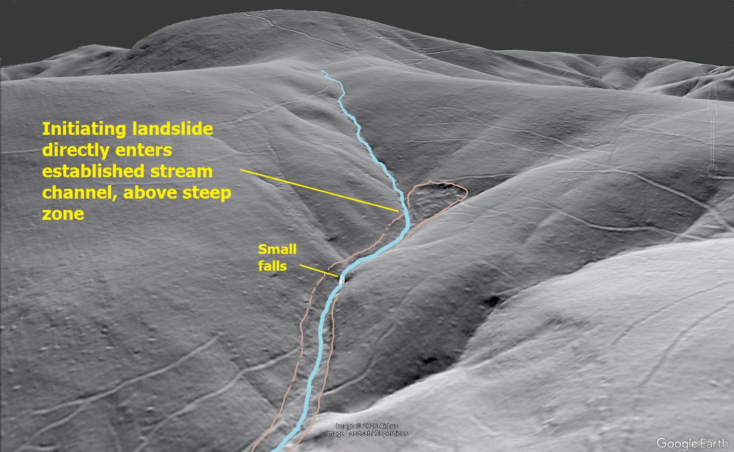
The Jacks Branch debris flow track remains clearly visible today, with significant scour occurring along a steep portion of Jacks Branch just below the initiating landslide.
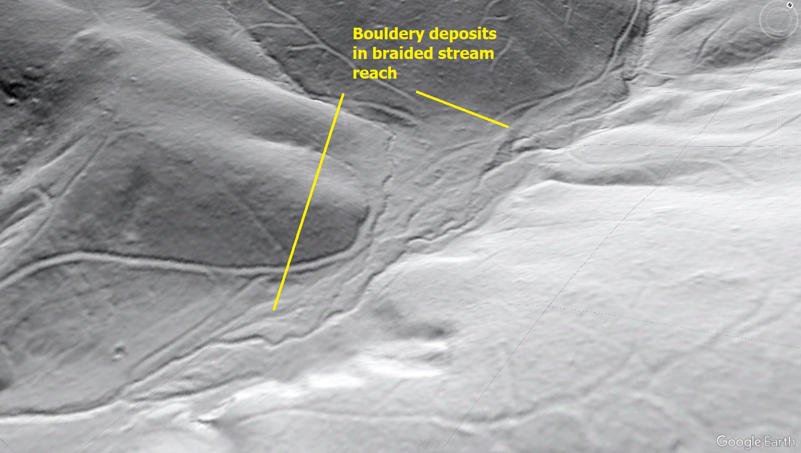
Below the scoured section, Jacks Branch has an almost braided appearance, with deposited boulders visible in 1-meter lidar imagery. The GIF below superimposes a 1/2 mile debris flow runout onto the lidar imagery, per description of the aftermath of the event recorded in 1916.
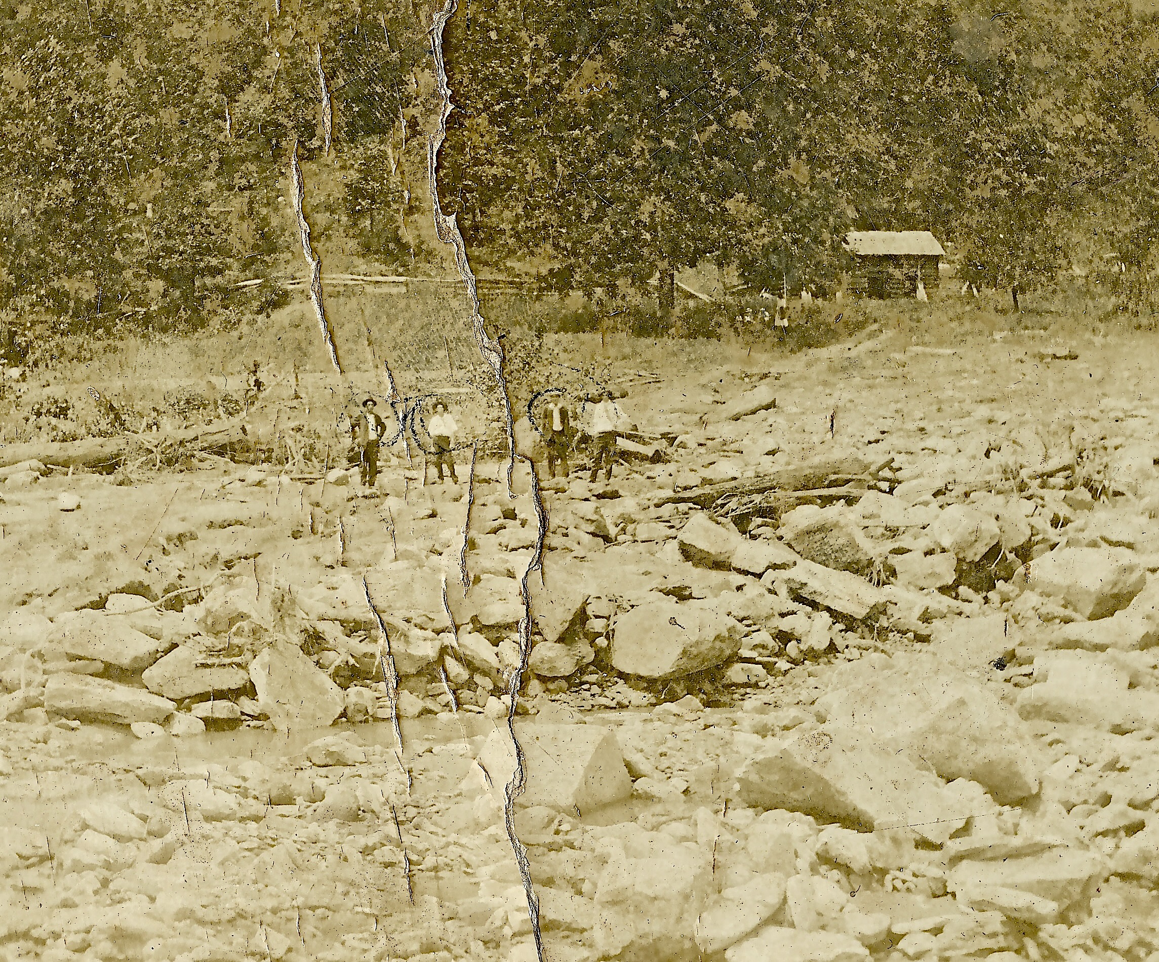
The 1/2 mile length appears to match the end of the braided channel and obvious boulder deposition fairly well, though a large amount of finer sediment likely continued downstream, mixed with floodwater. The lidar image below shows a detail of the bouldery ground surface, and the incredible 1916 photo, courtesy of Ann Loudermilk via Jule Hubbard, shows what the Jacks Branch aftermath looked like.
Locating this debris flow with lidar was initially a bit of a challenge due to the overall shape of the topography and atypical position of the initiating landslide. The scour of the Jacks Branch channel was the most useful identifier, whereas many debris flows of the higher Blue Ridge are first picked out by their initiating landslides within colluvial hollows. In the case of Jacks Branch, as with nearly all Appalachian debris flows, an initiating landslide triggers loading and liquefying of the saturated soil and rock debris along the channel downstream (more on this later). This “feedback” process produced an ever-growing mass of liquefied soil, rock, and trees, scouring the channel and delivering a huge amount of debris to the valley below. This GIF offers a conceptual animation of the process, along with the appearance of the aged and weathered track and deposit as it is seen in lidar imagery today.
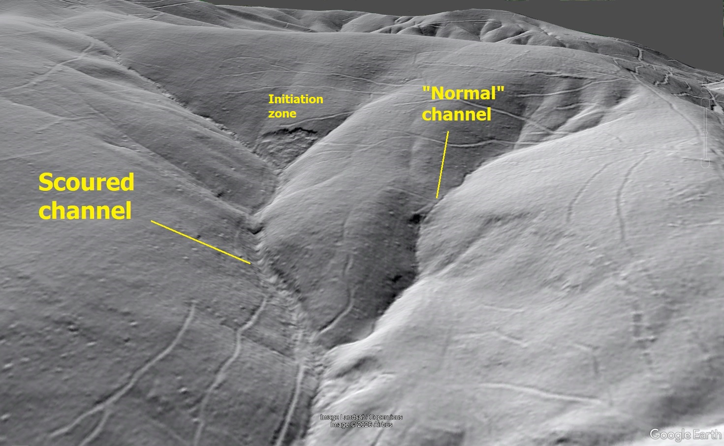
The scoured channel is quite impressive at 70 feet wide, even in the context of debris flows in the higher Blue Ridge that take advantage of longer, steeper slopes. The image below allows comparison of the scoured reach of Jacks Branch to an unaffected headwater stream. Prior to the debris flow, Jacks Branch likely presented a similar appearance.
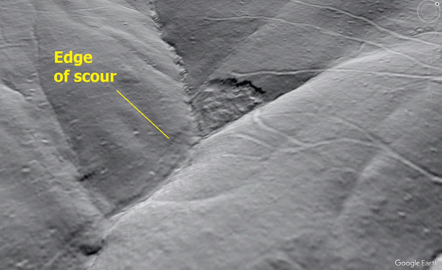
Scour can be seen cutting across the toe of the slope immediately below the initiating landslide.
The Jacks Branch debris flow seems large in its scale and runout for the host topography, but we admittedly lack a large number of comparative examples to support such a statement. A notable aspect of the debris flow is that its initiating landslide entered the Jacks Branch channel well below its headwaters, causing the slide to enter an established stream that would have been moving a large amount of water at the time of the slide’s occurrence. Introducing the slide to the high stream flow may have aided liquefaction and mobility, or the slide may have briefly dammed the stream before its lower portions liquefied and initiated the debris flow. This second option may explain why much of the initiating slide is left behind (lumpy area in the image above), as the initiating slide of most debris flows in the region liquefies upon movement and leaves an empty scar. In either case, the flow promptly descended a very steep portion of Jacks Branch, where it gained mass and energy and headed for the valley below.
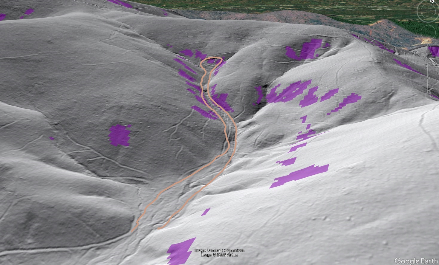
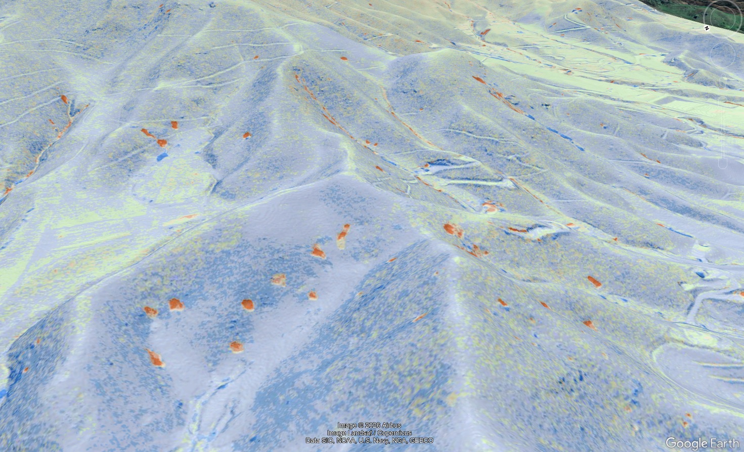
One detail that is lost to history (and can’t be answered from lidar imagery) is where the Russell cabin was located. One of Jule’s sources indicated that the cabin was located “on the mountain,” and not in the defined flat valley below. Somewhere near the confluence of the streams near bottom center of the image above is likely a reasonable location. The Russells obviously were not thinking about debris flows when they built or first occupied their cabin, and Jacks Branch or its tributary probably seemed too small to ever present a flood risk. I superimposed ALC’s Susceptibility onto the Jacks Branch area to see what we might say about building in this landscape today, given its distinctions from the high Blue Ridge. Areas where debris flows could potentially initiate (purple) do occur through the Jacks Branch basin, though in a somewhat different pattern from more rugged Blue Ridge landscapes. The Jacks Branch debris flow is outlined in brown.
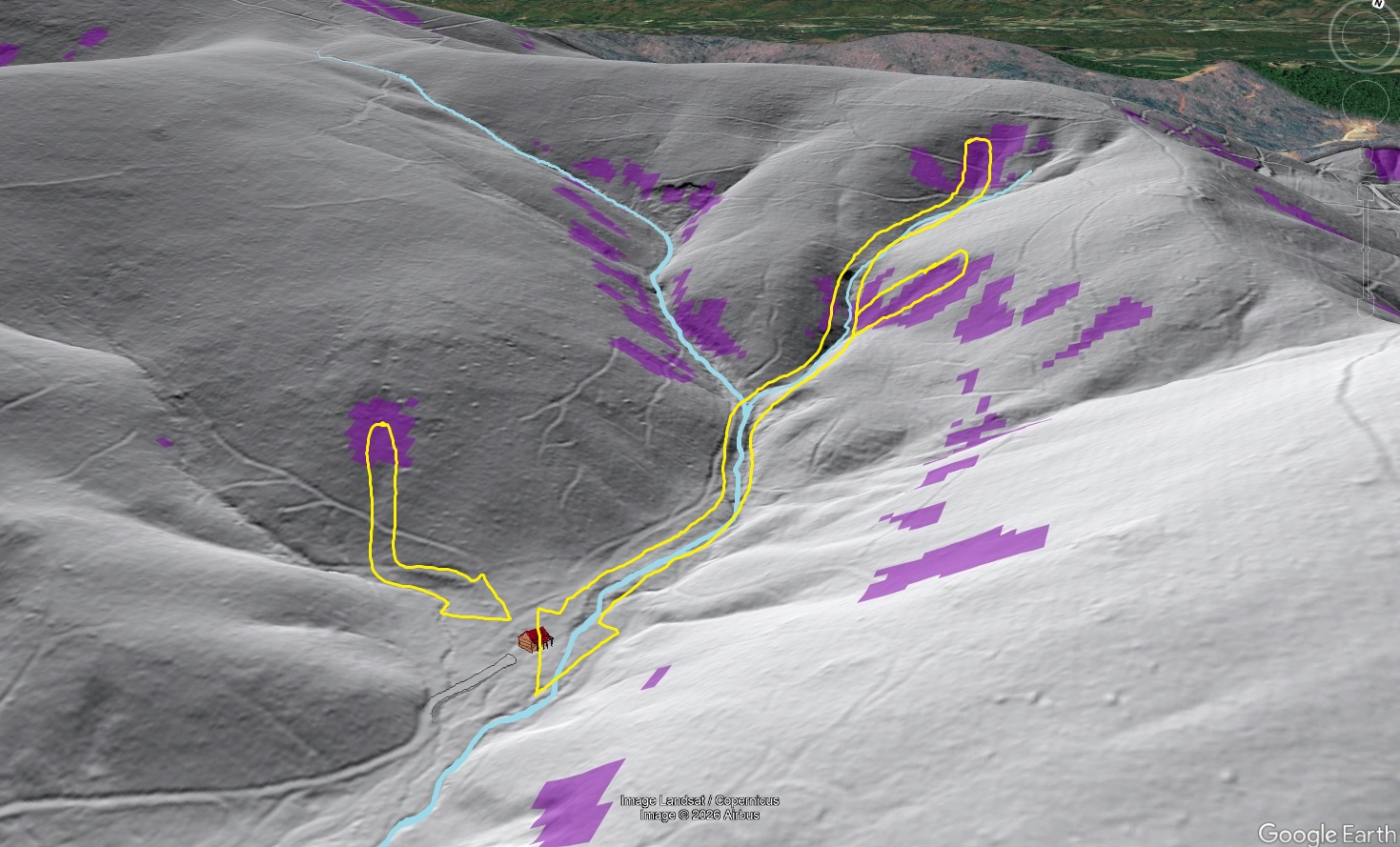
While this drainage basin is significantly less purple than many we look at, hazard areas are present, and debris flows initiating in them would follow the locally quite steep channels to the valley below. My pick for hazard the area shown above would be east (to the right of) Jacks Branch, in the steep, high hollows of the Jacks Branch tributary. A debris flow initiating there would ultimately end up in the same place as the 1916 debris flow, on the flat, deposit-filled valley below. While the flat valley area represents attractive, buildable topography that feels protected by the mountains, it’s quite vulnerable to debris flows during extreme weather conditions. The yellow arrows below show only a few of the possible debris flow pathways.
The Jacks Branch story is a valuable piece of history and an important lesson about steep slopes and extreme storms in the region. Huge mountains aren’t necessary for big landslide issues, particularly when rainfall and widespread soil saturation is sufficient to trigger debris flows. Debris flows tend to occupy MUCH larger widths than even the worst floods on the small streams they follow, leading to unbelievable aftermaths that suggest an impossibly huge “river of mud of rocks” suddenly appeared in a tiny valley. Linney’s account in the linked article communicates this idea very clearly. Avoiding the worst-case water flood on a small mountain stream isn’t enough if debris flow-prone topography is upstream.
Many similar stories undoubtedly exist in the region, and they all have their place in improving landslide awareness when the next “big one” hits, whether it is a tropical system or a one-off stationary thunderstorm. Anyone living in the mountains should take time to determine landslide hazard at their property and have a plan in place for when the “5 inches in 24 hours” threshold is likely to be exceeded.
New lidar imagery shows the full extent of Helene’s impacts
by Philip S. Prince
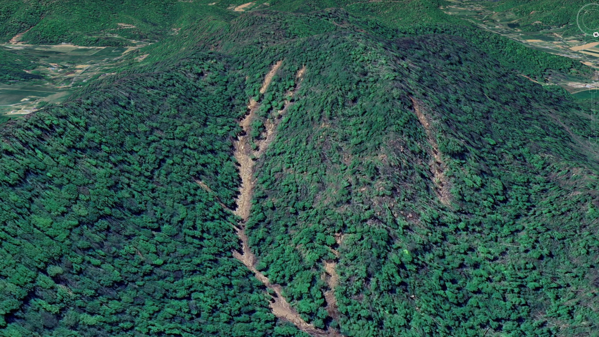
Over the last year, numerous collections of aerial imagery have shown Helene’s effects on western North Carolina mountainsides. This imagery has been useful in understanding the extent of the storm’s impacts on the landscape, but remaining tree cover and the natural irregularity of the landscape make it difficult to fully appreciate changes created by landsliding and flooding. Recently, long-awaited post-Helene lidar data has become available. Processing that data into imagery illustrating land surface by color coding loss and gain fully captures the storm’s effects. ALC Principal geologist Stephen Fuemmeler has produced county-wide change maps for Buncombe and Watauga Counties, and the results speak for themselves. The upper image below from the Big Ivy area of Buncombe County, North Carolina, shows Google Earth aerial imagery of debris flow landslides and tree blowdown. The lower image shows the same view with color-coded lidar surface change, highlighting debris flow scour and deposition as well as smaller landslides and the “divots” left by fallen trees.
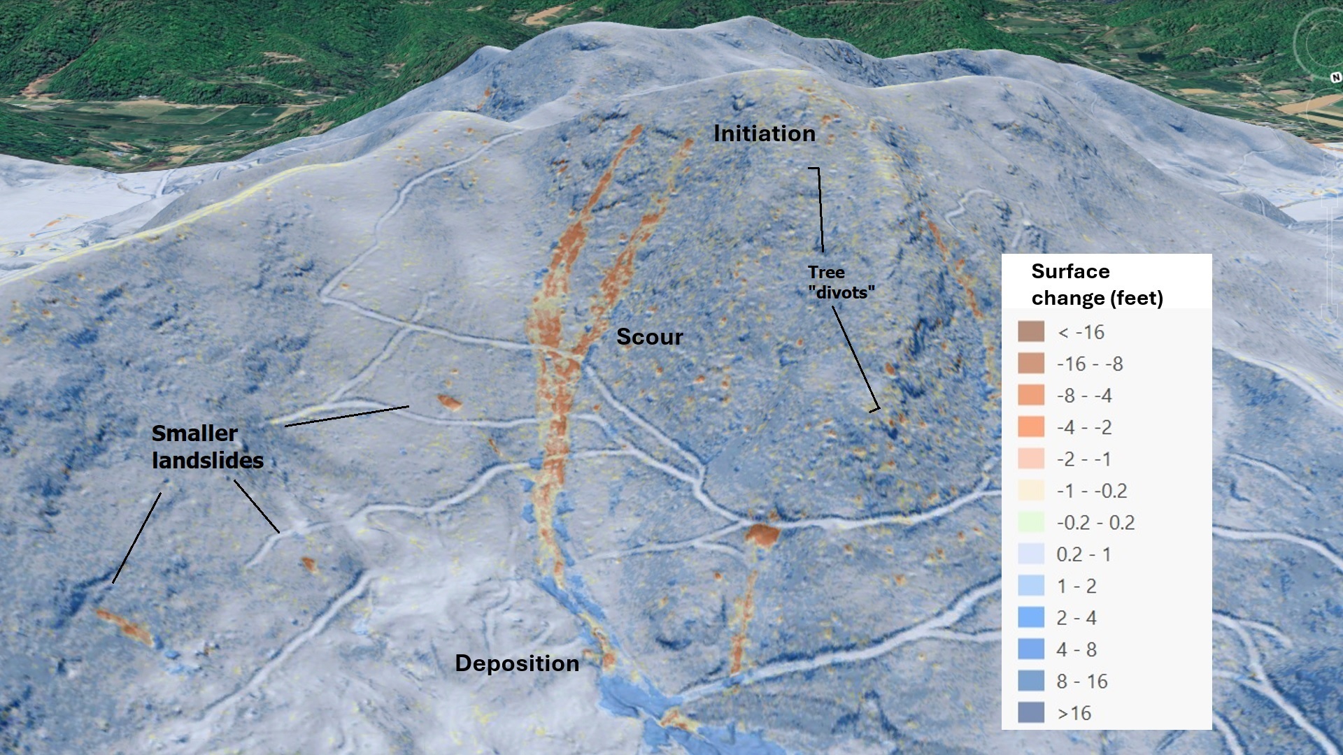
The lidar change imagery is a basic point-by-point elevation comparison from data before and after the storm. Areas lower after the storm are indicated by yellows to oranges (brown if really extreme); these are areas from which material was removed by landslide processes or water erosion. Blues highlight areas where the land is now higher from transported soil and rock debris piling up. The entire landscape is often faintly tinted due to miniscule mismatches in positioning pre- and post-data, so the combined loss (scour or down-dropping) and gain (piling up) pattern, the shape and context of identified changes, and the raw appearance of the new lidar imagery are all important for interpretation. The following GIFs give an idea of what the change patterns look like for a couple of landslide styles, starting with debris flow landslides that scour from an initiating slide and produce a deposit downslope.

The lightest yellows indicating minor change aren’t portrayed in the diagram to keep things simple. The basic pattern is a long, red-orange track where colluvial soil is now missing from being scoured away as it fluidized within the debris flow. The scoured soil ends up in a big, blue deposit where it piled up at the bottom of the slope. This pattern is nicely visible in the first change image in the post. A tremendous number of Helene’s slides fluidized due to soil saturation but didn’t scour the slope. These “blowout” slides were incredibly numerous, and have been of great interest to ALC over years of landslide mapping because they appear to associate with the most extreme rainfall events. A blowout change pattern is illustrated in the following GIF, which also includes a scouring debris flow (image center) for comparison.
Because blowouts don’t scour the slope, they appear as closed red or orange shapes, with the colored loss area produced by the scar on the slope. Many have a blue deposit pile somewhere downslope, but others don’t, suggesting the liquefied soil spread too thin for detection or reached a channel to be transported by floodwater. Fieldwork suggests that some blowout deposit material accumulated where transported woody debris lodged on standing tree trunks and began to trap soil.
Both of the conceptual models above are well represented by the Vanderpool debris flow and surrounding slopes in Watauga County, west of Boone.
In addition to the scoured track of the debris flow and its substantial deposit, a number of small blowouts are visible. Construction changes on the lower slopes indicate work done since 2017 and are not storm-related. The yellow arrow points out a small translational slide…more on this later. While the debris flow shown here was a monster that impacted downslope properties, blowouts were the big story in Watauga County, just as they were in 1940. They dot the image of the Sugar Grove area below. A small amount of deposit appears visible well below the red scars, reflecting the extreme mobility of the fluidized soil as captured on video in the area.
Blowout-style landslides are all over the Buncombe and Watauga landscape (the only counties I have reviewed so far), and many more have been observed in other impacted counties during fieldwork. Because blowouts don’t scour a track down the slope, they can be hard to detect from aerial imagery. The following example from the headwaters of Garren Creek in Buncombe County shows how well these slides hide in the remaining forest cover. The scar is an impressive 60 feet wide. It is faintly visible in the aerial imagery once you know it’s there. This failure would have sent an impressive wave of liquefied soil, along with the few trees sitting on the failed area, downslope at high speed. No deposit, with the exception of a couple of small lumps, is visible, indicating the fluidized soil made it to the stream below (out of the frame of the image). The “vanished” material also confirms the scar’s landslide origin. No spoil is present despite the large missing volume, and no well-traveled access path (or road!) is present to mobilize machinery or personnel onto the steep slope.
Debris flows and blowouts weren’t the only slope movements triggered by Helene (remember the yellow arrow in the Vanderpool example?). Movement of intact landslide masses occurred in many locations. Due to their limited displacement, these slide movements are difficult to detect without the aid of lidar change analysis….unless one is in your backyard. Intact slides produce their own pattern of surface elevation loss and gain, with the downslope toe of the slide uplifting to various degrees as upper portions of the slide drop down along headscarps and internal scarps.
Many of these larger, slightly moving slides were reactivations of older slide features developed in huge colluvial accumulations around the flanks of steep slopes. The following images from the south side of Watch Knob, west of Swannanoa at the mouth of Bee Tree Creek, show a couple of large, intact slides. The GIF compares 2017 (pre-storm) lidar, 2025 post-storm lidar, and lidar change detection. Headscarps locations are indicated by yellow arrows; the headscarps appear as the second panel fades in. Note construction-related change at lower left, below one of the big slides.
In addition to smaller landscape details, the physical scale of the larger debris flows triggered by Helene is captured by the lidar change products. The image below shows part of the eastern prong of the Craigtown debris flow complex. The combined total length of the orange scoured tracks approaches 1.75 miles, with consistent scour depths of up to 4 feet along that entire length. Intermittent scour (with limited local deposition) continued to homes that were struck at the base of the mountain. The sheer volume of material that moved here during the three pulses over 15 minutes is staggering…and this image only shows part of it.

Lidar change imagery is also useful for understanding how landslide material moves in a storm like Helene. Some fluidized slide debris, like that from Craigtown or many of the blowouts, is incredibly mobile on both open slopes and in headwater channels. Other debris flows show less scour and mobility, despite developing from substantial initial landslides. The slide below occurred in the Big Ivy community. The upslope scar is 92 feet wide and exceeds 8 feet in depth at its center. Very limited slope erosion occurred as the initial slide debris traveled downslope, and impressive piles of deposited material developed where the landscape flattened slightly atop older, accumulated slide deposits. Whether the landscape or soil/rock characteristics reduced runout of this debris flow is unknown, but could possibly be determined through modeling and field study.
The debris flows below, from Buncombe County just west of Shope Creek, showed similarly short runouts, possibly due to topography and geology of the local ridge-forming rock from which colluvial soil is derived. The image uses the same scale change as above.
In addition to informing future modeling and hazard assessment, lidar change imagery also highlights areas that may need monitoring in future storms. The Watauga County slides at the center of the image below deposited material in a steep topographic draw, where it may be prone to saturate and fail again or be entrained by a future debris flow. Numerous examples of slide material ended up in potentially unstable locations can be identified easily, and these areas may need remediation attention.
Several geologists could devote the rest of their careers to this new lidar data and never run out of things to learn. You’ll see change results from Buncombe, Watauga, and other counties in posts on this page, and we’ll also be using them to inform fieldwork and planning in the coming months and years. As for the currently estimated 2,000 + landslides from Helene, it’s definitely on the “+” side of that…by many, many times!
The undeniable value of landslide risk assessment
Landslides (and particularly debris flows) aren’t a daily occurrence in western North Carolina, so knowledge of the landslide risk of a specific property may not always seem important. A few years ago, ALC advised a client against purchase of a high-risk property located in an area that, at the time, seemed quite safe and desirable for a mountain home. The risk potential of the property turned into devastating reality during Helene, and a significant loss was avoided thanks to the pre-purchase site evaluation and subsequent decision to buy and build elsewhere. The locations and images of the impacted property are described in this post with the client’s permission. Her experience is noted in a Garden and Gun article linked here.
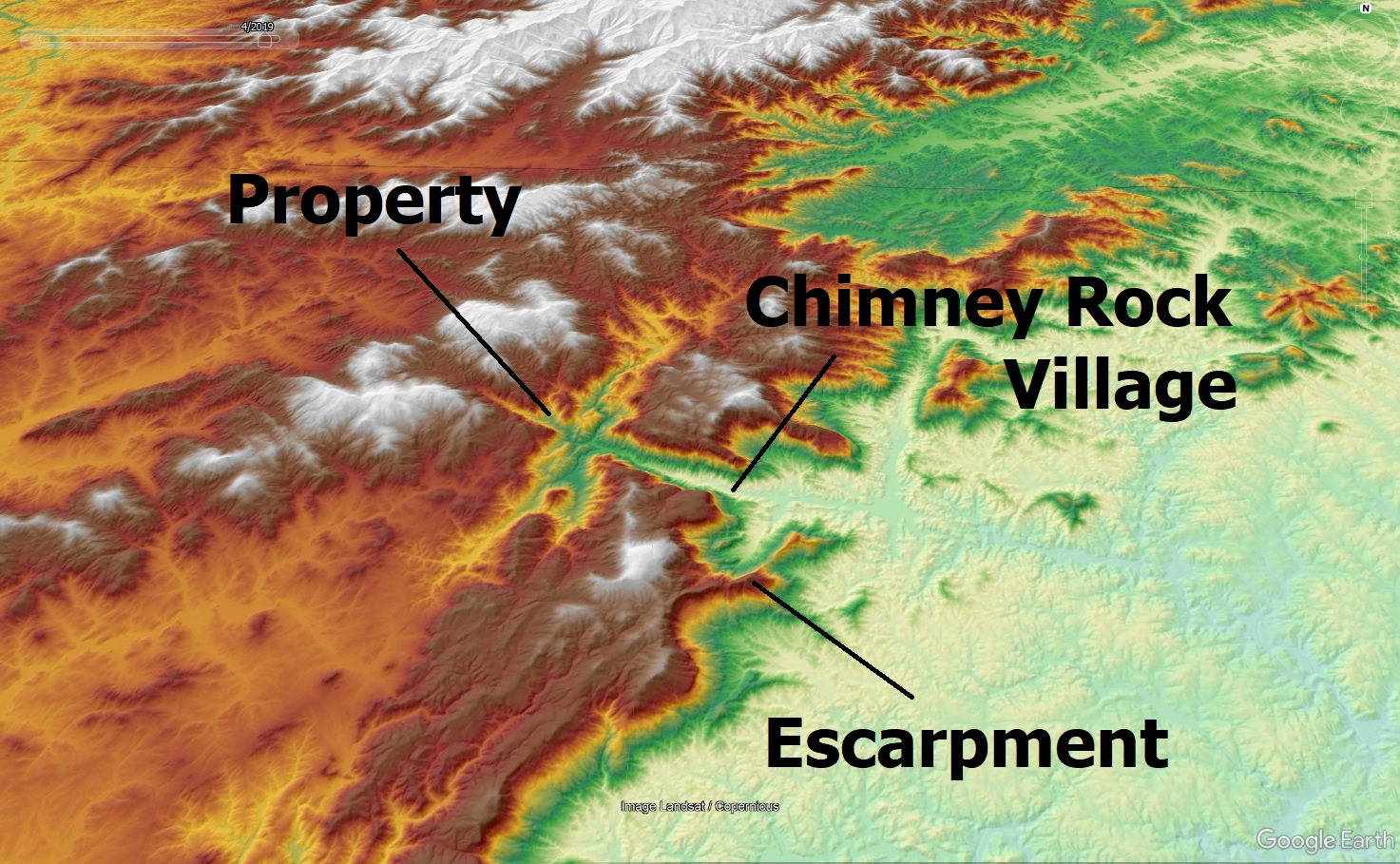
The impacted property is located immediately adjacent to Middle Fork, a tributary to Hickory Creek just upstream of Bat Cave, North Carolina.
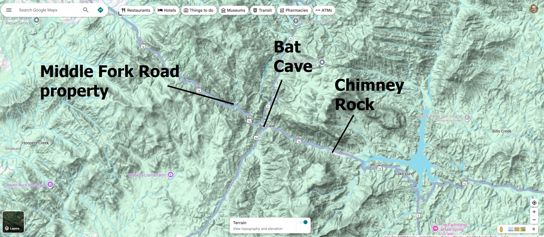
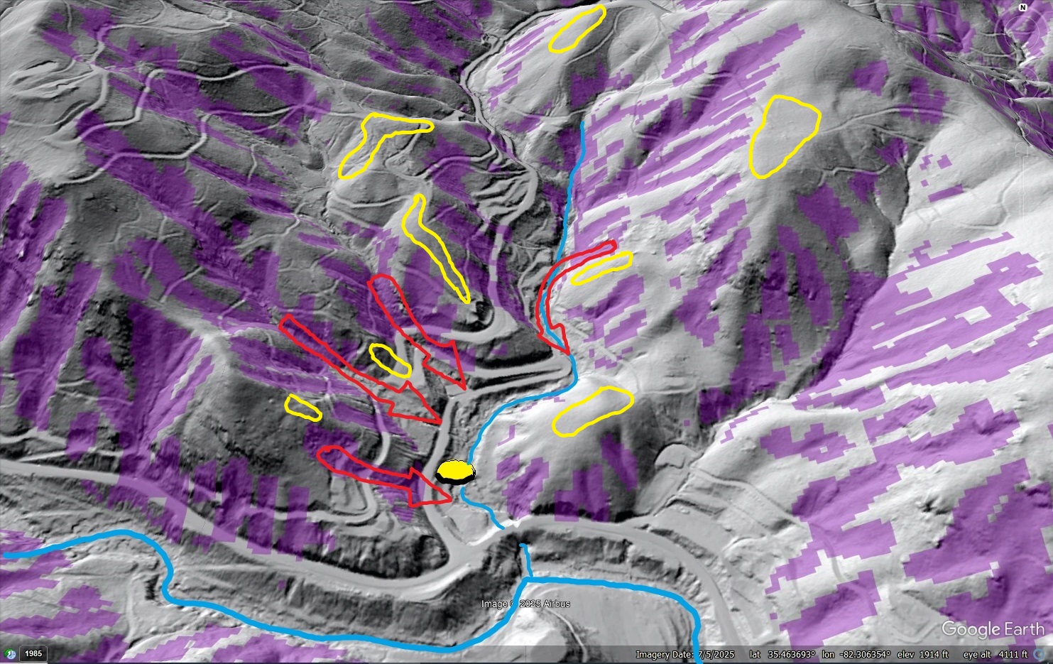
The location raised immediate concern during ALC’s evaluation because of the property’s potential to be impacted by both debris flows and flash flooding. A known debris flow occurred just northwest of the property (yellow outline below), nearly reaching it. The property itself is located in mapped landslide deposits (orange outline), and numerous potential debris flow initiation areas (purple) were identified upstream of the location by ALC’s Susceptibility Model.
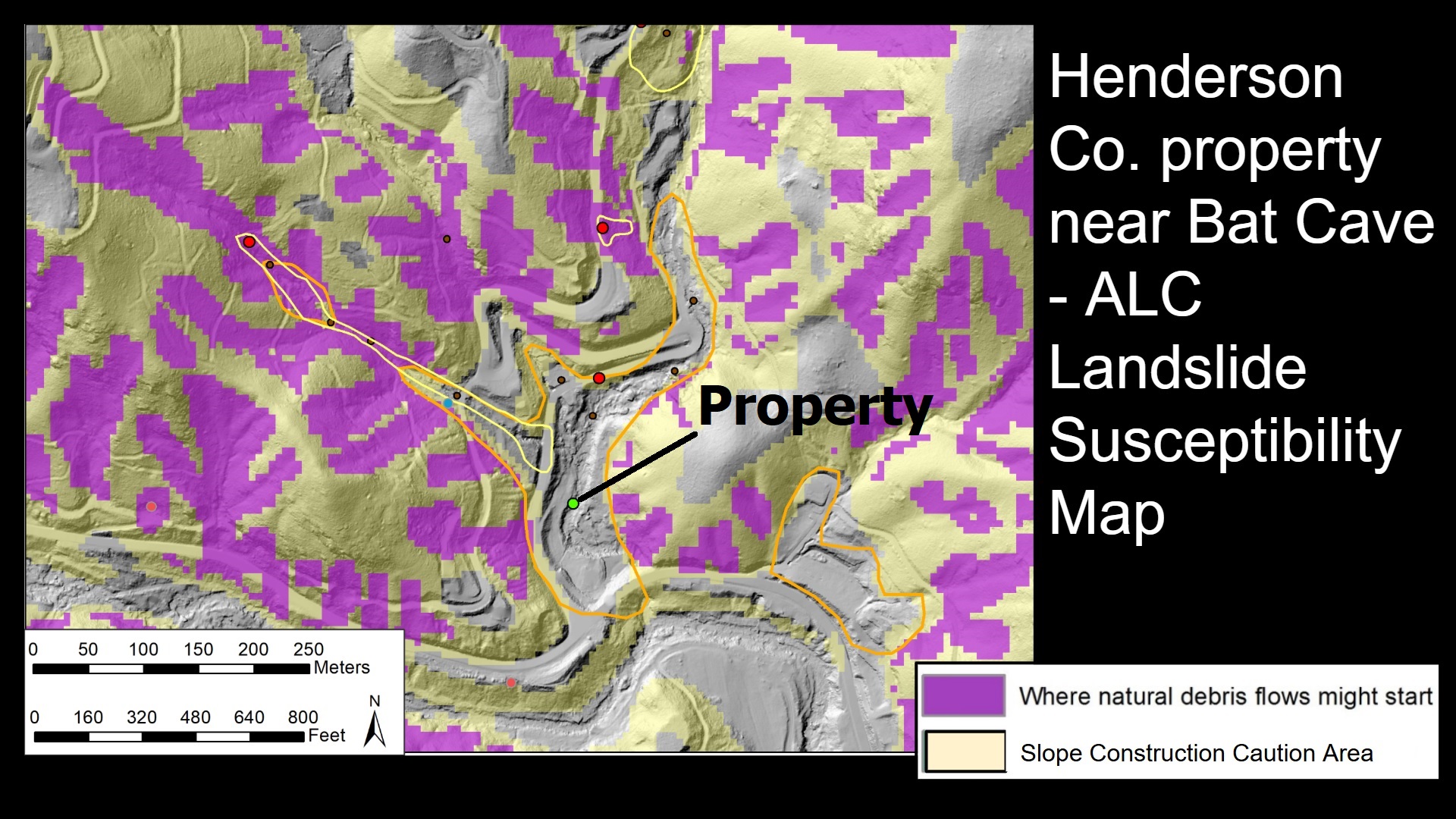
Debris flows are exceedingly mobile and can transition into more flood-like features as they travel down streams and mix with runoff, extending considerably the potential reach of debris flow hazards from potential source areas. Even without landslides that develop into debris flows, the potential for flash flood impact on the property was significant. The property is located on a streambank in a small gorge in the Blue Ridge Escarpment Zone, where topography can force air masses to rise and produce extreme localized rainfall.
This rainfall, combined with the steep topography, quickly makes normally tiny streams very dangerous. The location in question would, eventually, see the effects of an extreme storm event. The only question was when this would happen.
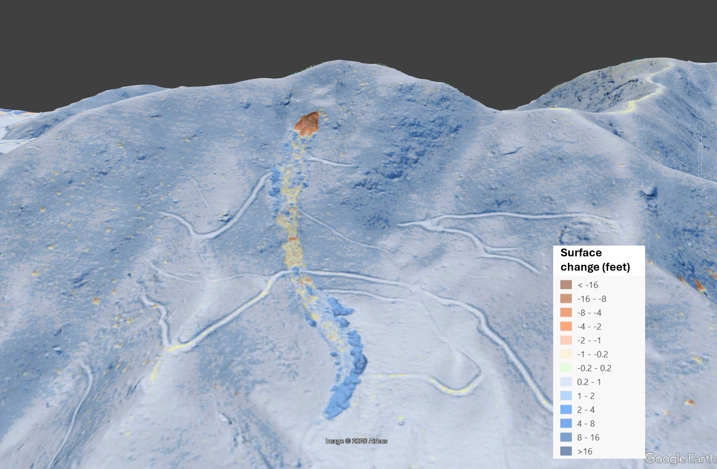
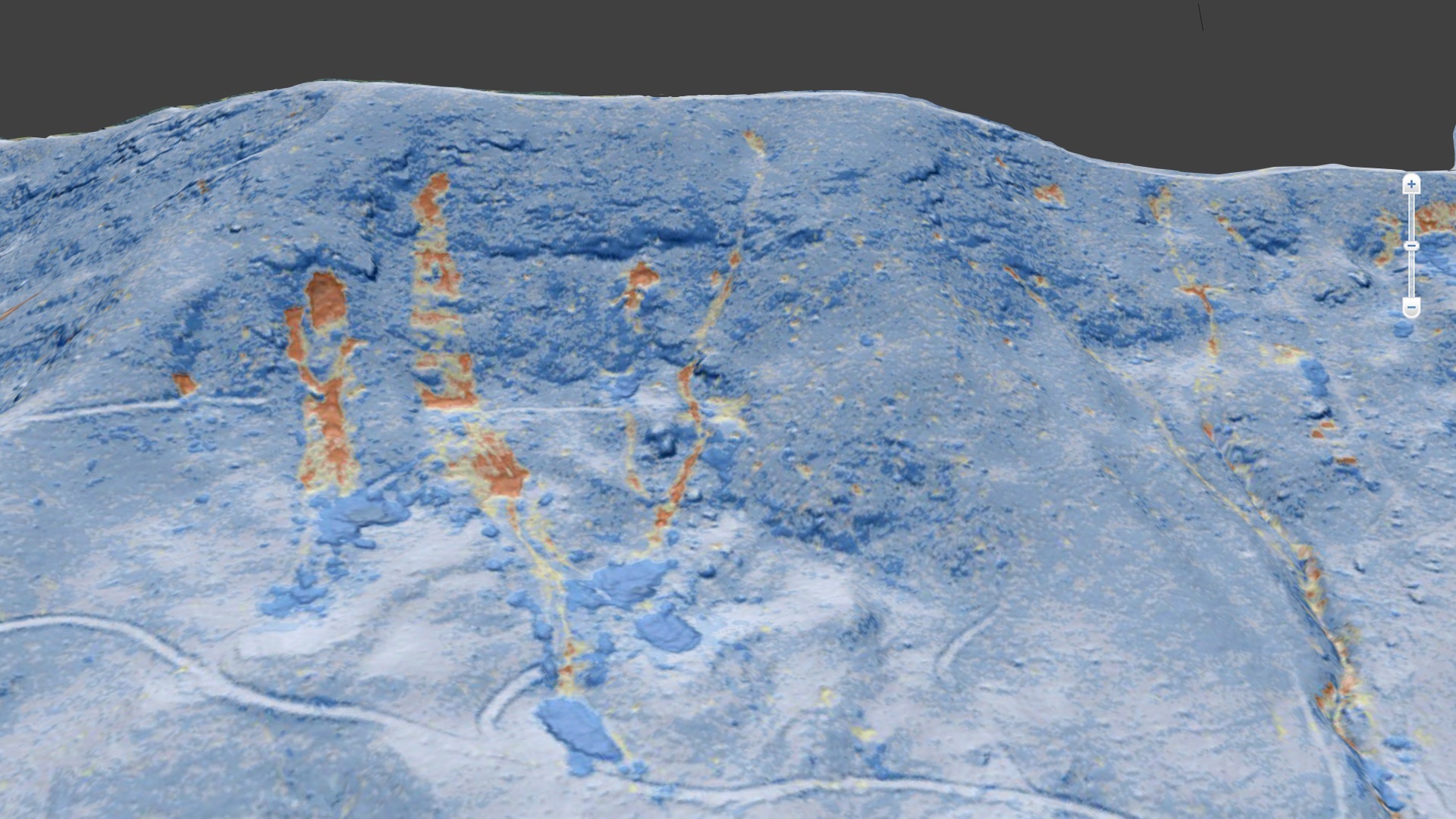
ALC recommended that the client seek another property for house construction. The streamside, off-the-beaten-path location was indeed desirable, but the potential for severe impact across the entirety of the property was too great. While the Middle Fork property could have daytime recreational value, living (particularly sleeping) there and investing in a structure on the site was too great a risk. In September 2024, Helene showed just what that risk looked like. The top image shows the site before Helene; the bottom image is the same view after the storm.
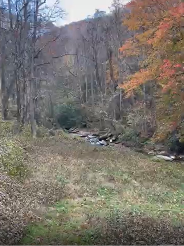
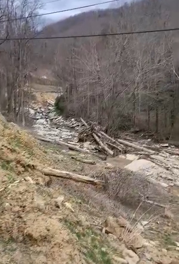
Both significant debris flow events and record flooding affected Middle Fork, scouring the property and leaving enormous piles of debris behind, including huge, mature trees mobilized by debris flows and floodwaters. A structure on the property would have been a total loss, and anyone inside during the peak of Helene’s impacts would have faced serious injury or death. The GIF below compares pre-Helene, 2023 imagery to post-Helene imagery. The property location is shown by the large yellow arrow.
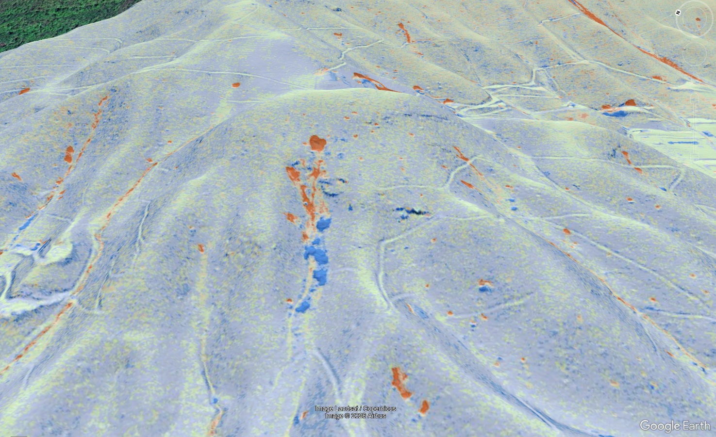
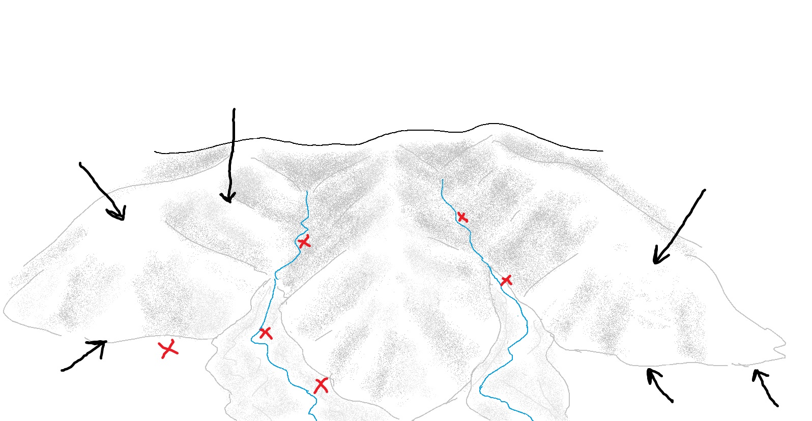
Fortunately, the client heeded ALC’s recommendation and purchased well-situated property in Yancey County, which avoided damage due to its position within the landscape despite Helene’s catastrophic impacts in Yancey. The hazard potential on both the selected Yancey property and the Middle Fork property were evaluated remotely–simply looking at detailed topographic maps, lidar imagery, and records of past debris flow events painted a clear picture to geologists with years of experience in the region. In this case, the return on investment in the evaluation was quite significant, with the client able to avoid a major loss and instead devote resources towards a property in a more stable and resilient location. The fundamental concept behind this type of evaluation is being able to read the landscape shape and history and visualize impact potential. The images below illustrate the concept. Black arrows show locations where convex slopes (and often elevation) steer debris flow and flood hazard away; red X’s are in areas to which debris flow and flood hazards are directed by landscape shape.

Landslide risk evaluations aren’t meant to show that entire regions are unsafe for building and living. Because debris flows and floods follow the terrain as fluids (water and liquefied soil both run downhill), their potential impact zones are limited. Even along Middle Fork, numerous safe and livable areas exist along convex portions of the landscape that shed flowing material instead of focusing it. Yellow outlines in the image below show examples of these areas–in this topography, they are noticeably on ridge tops and “noses” of slopes. That said, road networks to access those safe areas are still vulnerable, and anyone choosing to live in them should be aware that access may be difficult or impossible after a major event. Even areas with landslide and flood hazard have conservation and recreation potential, though they should not be disturbed by development and must be avoided during hazardous weather.
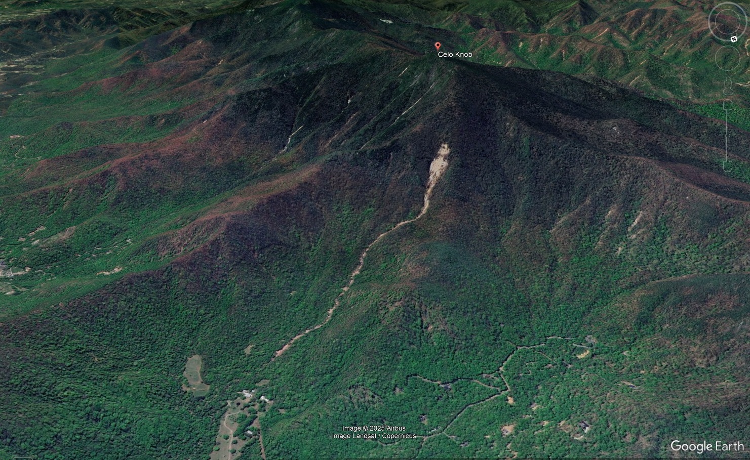
Interestingly, the Garden and Gun article inadvertently showcases another notable Helene event: the Celo Knob debris flow, which might have left the largest single scar (in terms of surface area) of any debris flow during the storm. The scar is visible in the background of the image below, which is from the article.
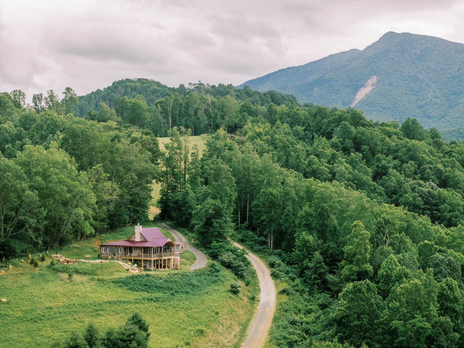
The clearly visible scar is 330 feet wide and 700 feet long from head to toe. The flow carved a nearly 5,000 foot long track down the mountain before running out of energy. The house visible near the terminus of the debris flow is somewhat above and away from the channel followed by the flow. It is uncertain whether the house could be impacted in a “worst case” debris flow event, or if such an event is even possible in the near future since so much material already moved. The scar of this huge debris is yet another valuable reminder of the importance of knowing what can happen under the right (or wrong!) conditions.

The 1847 debris flow event in Clay County, North Carolina shows crazy storms aren’t a new thing for the region
Seeing the results of past extreme storms in a region is an important part of understanding potential landscape behavior. Thomas L. Clingman (yes, that Clingman) provides an invaluable record of a couple of past storm events in his extensive writings about western North Carolina. His discussion of the results of a storm of July 7th, 1847, in Clay County is particularly interesting. The document is linked here, but the excerpt below contains the important parts found on page 76 of the document. Anyone that saw the effects of a Helene debris flow will quickly recognize exactly what Silas McDowell described to Clingman.
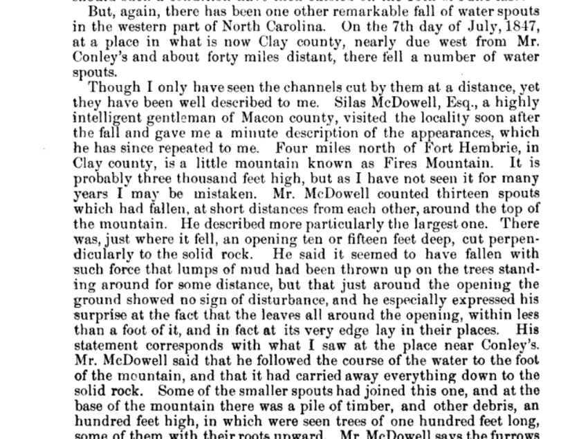
McDowell was very clearly describing debris flows to Clingman (not “waterspouts” as we use the term today), and Fires Creek Mountain was obviously hit with an impressive cluster of them during this storm. Because debris flows visibly scar the landscape, could a geologist still see the effects of the storm on Fires Creek Mountain nearly 180 years later? I took a stab at this a few months ago, and I was impressed at how well the combination of Clingman’s notes and 21st century lidar imagery worked together.
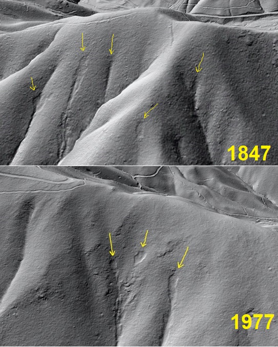
If you want to go looking for 180 year old debris flows, you need to know what sort of scars you might be looking for on mountainsides. An effective way to do this is to examine the lidar-visible scars of known debris flow events. The November 1977 storm produced quite a few debris flows southwest of Asheville in the Bent Creek area. These were captured in 1982 aerial photography when their scars were still visible in the forested landscape. These air photos can be matched to lidar imagery to directly confirm what debris flow scars look like in the landscape. The GIFs below show this process, with yellow arrows indicating the upslope starting points (initiation zones) of the debris flows.


Debris flows like these begin as an initial landslide, producing a distinct scar in the landscape with steep, sharp edges where the slide began. This scar transitions into a visibly scoured track where the debris flow rakes saturated soil from the slope in its path, adding to the flow’s mass. The GIF below gives a general idea of this starting process and the scar that it makes, from the initial slide to the early phases of scour.

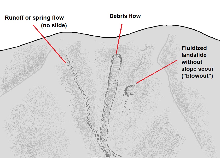
Within the grayscale world of lidar-derived hillshade imagery, debris flow scars can be distinguished from small, water-carved channels due to the effects of the initial sliding and subsequent scouring processes. Fluidized landslides similar to debris flows, but without the long, scoured track (referred to as “blowouts”), also produce distinct scars. The sketch below offers a basic summary of what you’re after as you peruse lidar imagery.
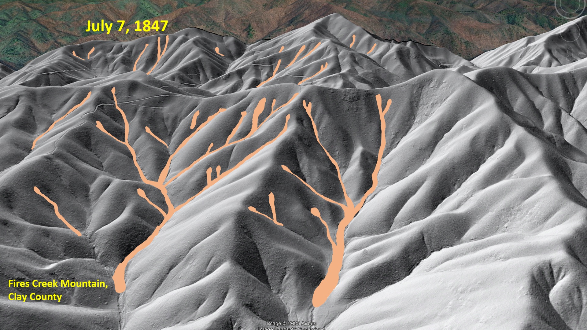
So, with this knowledge in mind, it’s time to take a look at Fires Creek Mountain. Clingman’s geography and distance estimates are always excellent, so I drew a line four miles due north from the Fort Hembree historical marker’s general area. The line met the top of Fires Creek Mountain at about 3.9 miles in a debris flow-susceptible area…not bad. The lidar imagery does the rest.
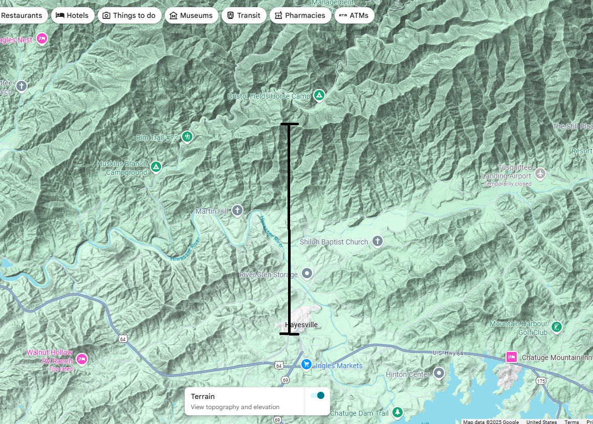
There are indeed an impressive number of debris flow scars on Fires Creek Mountain at the top end of the black line, exactly where they should be. Their appearance is unmistakable, and they distinctly cluster within a limited area as Clingman notes in his report. Yellow arrows point them out below; many more are visible in the zoomed-out view that follows. They aren’t labeled in the large view–see how many you can find.
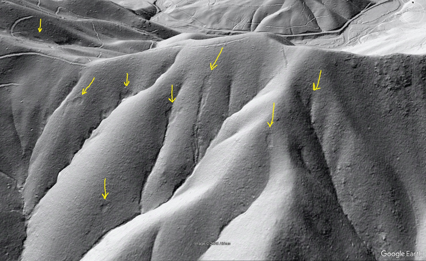

The scars are well-preserved and look like the 1977 scars, though a bit worse for wear after 180 years.
This 1847 storm was likely an isolated storm “stuck” on the mountain ridges, given the limited size of the most intense debris flow activity. Clingman references observers in the valley below watching the storm on the mountain but not experiencing the intense precipitation themselves. Had this storm happened today (or in the era of easy photography, particularly aerial photography), it would have been intensely documented and firmly cemented in local lore. Today, it might make international headlines, particularly if someone caught a video of one of the debris flows reaching the valleys. How readily visible the debris flows and blowouts were from the valley below in 1847 is hard to know, but it was obviously eye-catching enough to have attracted attention and investigation from locals at the time. The images below show brown outlines over the visible features.

Extreme storms are likely to become more common in a warming atmosphere, but they’ve always been a part of the southern Appalachians. Helene’s impacts were exceedingly widespread, but more localized–and more intense–storms have happened in the past and will continue to happen in the future. It’s worthwhile to look back on these events and their impacts as a reminder that all sorts of things can happen in our region when conditions are right.
What happened to mountain slopes during Helene? Geologists are gathering information to prepare for the next storm

In the nine months since Helene’s arrival in western North Carolina, geologists have worked steadily to better understand how to reduce future landslide-related impacts on life and property. While landslide themselves cannot be prevented from happening under extreme precipitation conditions, decision making during, and particularly before, a storm can save lives and reduce damage to infrastructure and personal property. Understanding what made certain landslides more damaging than others requires both extensive fieldwork and study of remote sensing data, like lidar imagery. ALC Principal Geologist Jennifer Bauer and Project Geologist Philip Prince recently presented some of the findings of their post-Helene work in US Geological Survey seminars. Video recordings of the talks are linked below. If you have ever wondered what a geologist sees in one of Helene’s thousands of landslide scars, these videos will give a glance of how we do our work day-to-day.
Jennifer Bauer
Jennifer’s talk focuses on the use of landslide mapping and modeling to understand and (more importantly) communicate landslide hazard before storms hit. Understanding landslide potential in a given landscape requires that geologists understand the landslide history of a landscape. Landslide inventories involving both lidar imagery analysis and lots of boots-on-the-ground fieldwork help geologists learn what has happened in the past.

Once the geologic details that can produce landslides are understood (slope shape, slope steepness, soil type, etc.), models of potential landslide hazard zones can be developed. As Jennifer’s talk shows, the overwhelming majority of Helene’s landslides came from mapped hazard areas, but not every hazard area produced a landslide…this time. Hazard mapping can show mountain residents areas that are potentially dangerous is storms (don’t worry; it’s not everywhere-not even close) and help with decision making regarding where to live and how to prepare for the next big event.
Philip Prince
Philip’s talk is centered around the geologic details of Helene’s debris flow landslides. Debris flows are fast-moving, fluidized landslides that can travel long distances very quickly. Often called “mudslides,” debris flows actually carry huge amounts of rock and boulder debris and tremendous numbers of trees, so a debris flow impact is much more damaging than what might result from mud alone.

Philip illustrates where debris flows start in the landscape and how they accumulate so much material on their path downslope. A large debris flow could cover a football field with a few feet of mud, rocks and trees, but even small debris flows are surprisingly destructive. By understanding what type of geologic materials and slope settings produced debris flows during Helene, we can better understand what areas may be hazardous in the next event. Planners can also what parts of the landscape may be more susceptible to landslides when disturbed for building, as well as what areas at the foot of the mountains might be reached by debris flows.

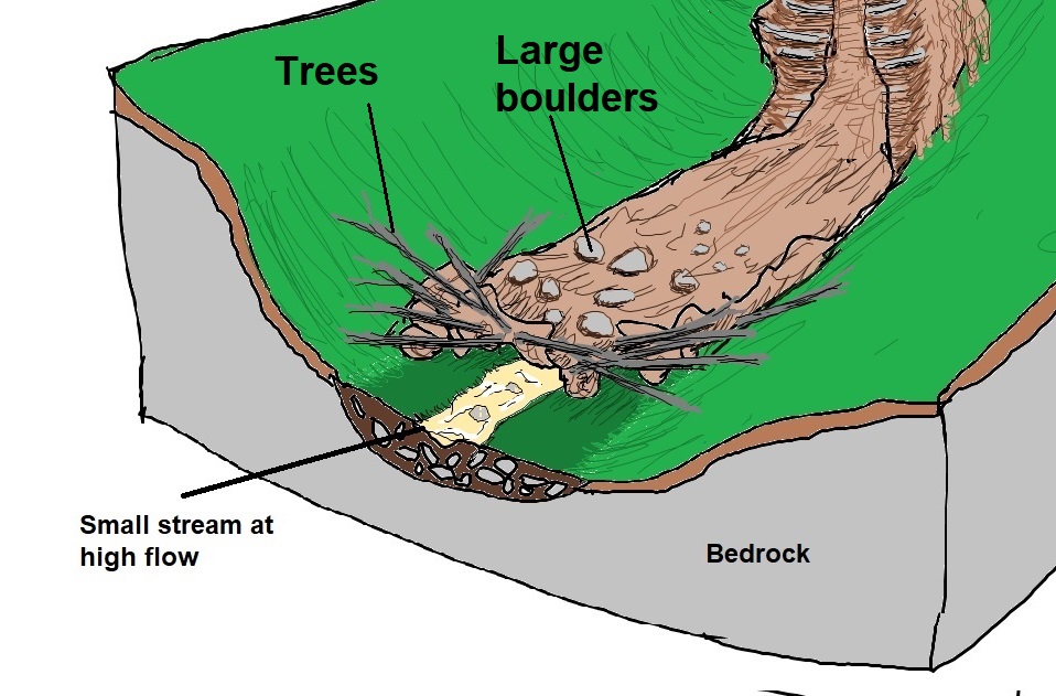
Understanding debris flow landslides in the southern Appalachians
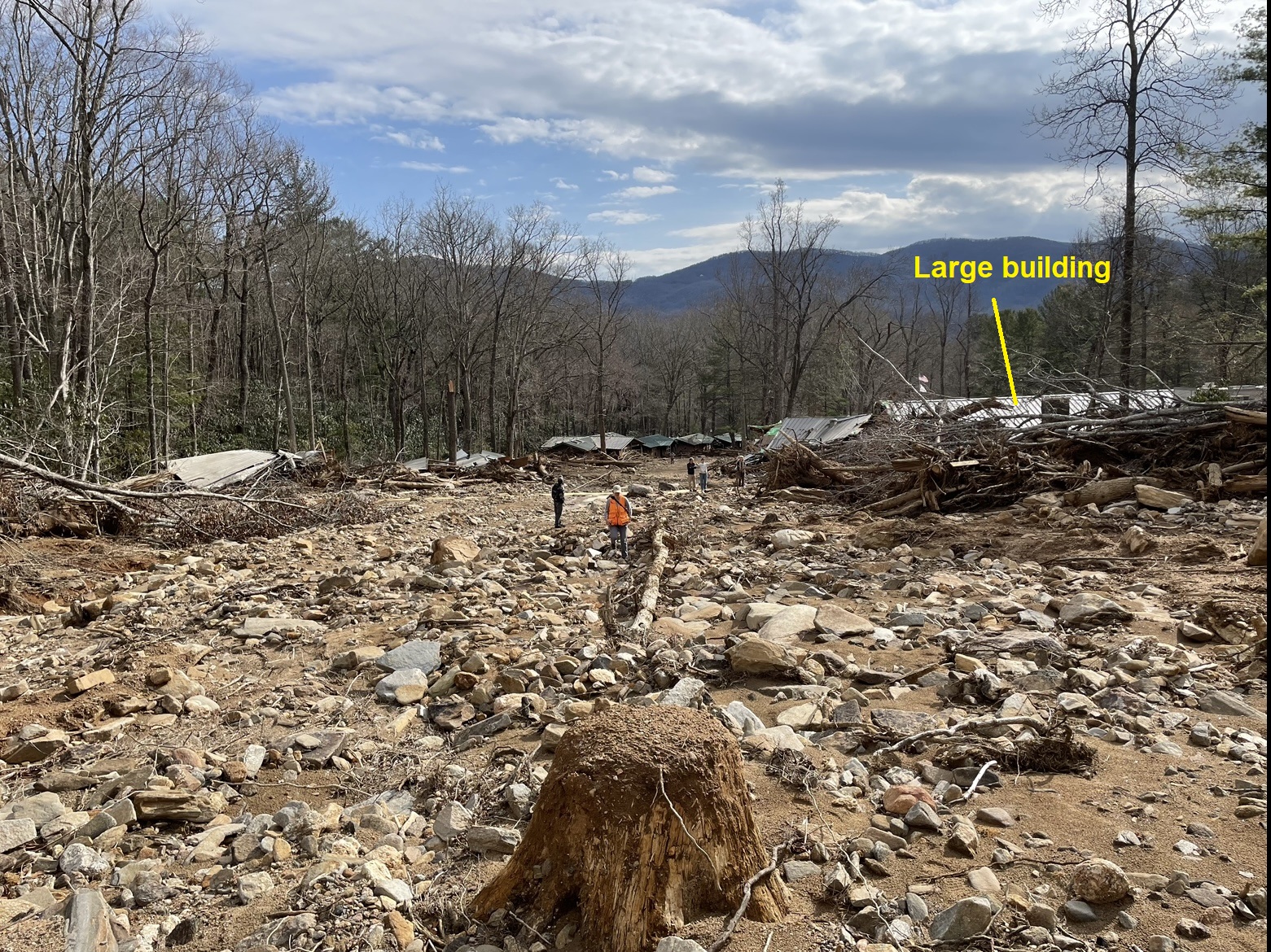
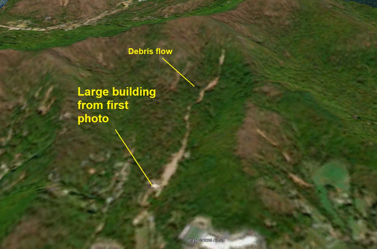
Before Helene’s remnants passed through western North Carolina, the boulder-strewn area in the photo above was covered with trees and buildings. A small stream flowed behind the wrecked buildings on the left of the photo. The damage seen here occurred suddenly on the morning of Friday, September 27, 2024, as a huge wave of boulders, trees, and mud surged down the small stream’s channel. This wasn’t a flash flood–it was a debris flow, a type of fast moving, fluidized landslide associated with heavy rainfall. The extent of the damage from the debris flow is visible in the before/after GIF below. The photo above was taken near the top of the GIF images, looking towards their bottom. The large building labeled above is visible near the bottom of the GIF images.

The small stream is visible trickling through the damage swath; water flooding alone from a stream this small could never approach the level of damage caused by the debris flow. Fortunately, no one was seriously injured in this particular debris flow, but many lives were lost in similar events elsewhere during Helene. Understanding these particularly dangerous landslides is a big part of storm safety in southern Appalachia. So, what are debris flows, where do they start, and what makes them so dangerous?
What are debris flows?
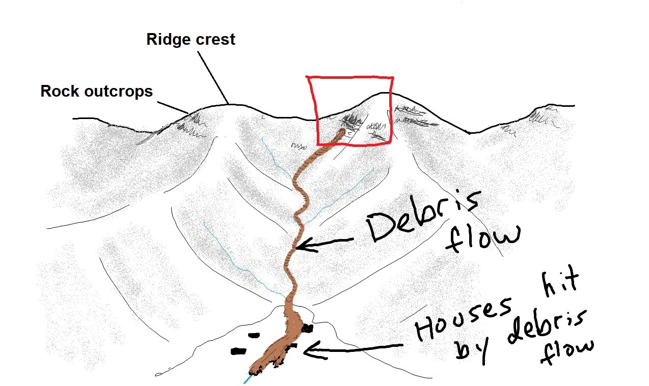
Debris flows are fast-moving, highly mobile, fluidized landslides transporting saturated soil, boulders, and trees downslope. They are specifically associated with saturated soil, which results from heavy rainfall in our region. Debris flows move like a liquid but contain large amounts of solid material–65% solids (rock, soil, and wood) is an average composition, with the rest of the flow volume being water mixed into the soil and rock. Often called “mudslides,” debris flows also carry large trees and boulders. Because of their solid content, debris flows are approximately twice as dense as water, so they hit with destructive force. They follow ravines and small stream channels downslope due to their fluid consistency, spreading over wider areas at the base of slopes until they lose their momentum. The sketch below gives a general idea of a debris flow’s start-to-finish journey downslope, from its beginning in a steep hollow to its damaging end on flatter ground at the base of the mountain.
Where and how do debris flows start?
Debris flows frequently start in steep hollows, or slightly concave slope areas, above the headwaters of small streams. They can also begin on road embankments, or any other landscape feature that can initiate a small landslide on steep ground. Debris flows are specifically associated with heavy precipitation and saturated ground. When a landslide starts in saturated soil, it liquefies and accelerates. When the liquefied landslide hits the saturated soil in its path, this soil liquefies as well and is added to the debris flow. Much like a snowball, debris flows accumulate more and more debris moving downslope, adding to their volume and destructive power. The GIF below shows the basic idea of debris flow initiation in an area like the one indicated by the red box in the sketch above. Note that the debris flow starts in rocky soil beneath a cliff, where rock fragments have accumulated to the point of instability. Due to saturation, once the slide starts, it liquefies, and then liquefies the soil in its path.
How do debris flows move?
Debris flows follow ravines and stream channels due to their liquefied condition, typically scouring large amounts of soil and stream sediment on their way down. Moving within the stream channel keeps the flow confined and intact. Collisions between soil and rock particles help keep the flow liquefied. A confined, thicker flow also loses less of the water trapped within it. Debris flows can move very quickly, often at speeds of 20 mph or more. They frequently run up onto the slope on the outsides of bends due to their speed. Their width greatly exceeds the width of the stream or creek whose channel they follow. The conceptual sketch below illustrates the scouring process as well as debris flow size relative to the “usual” stream in the channel, even during high water flow.

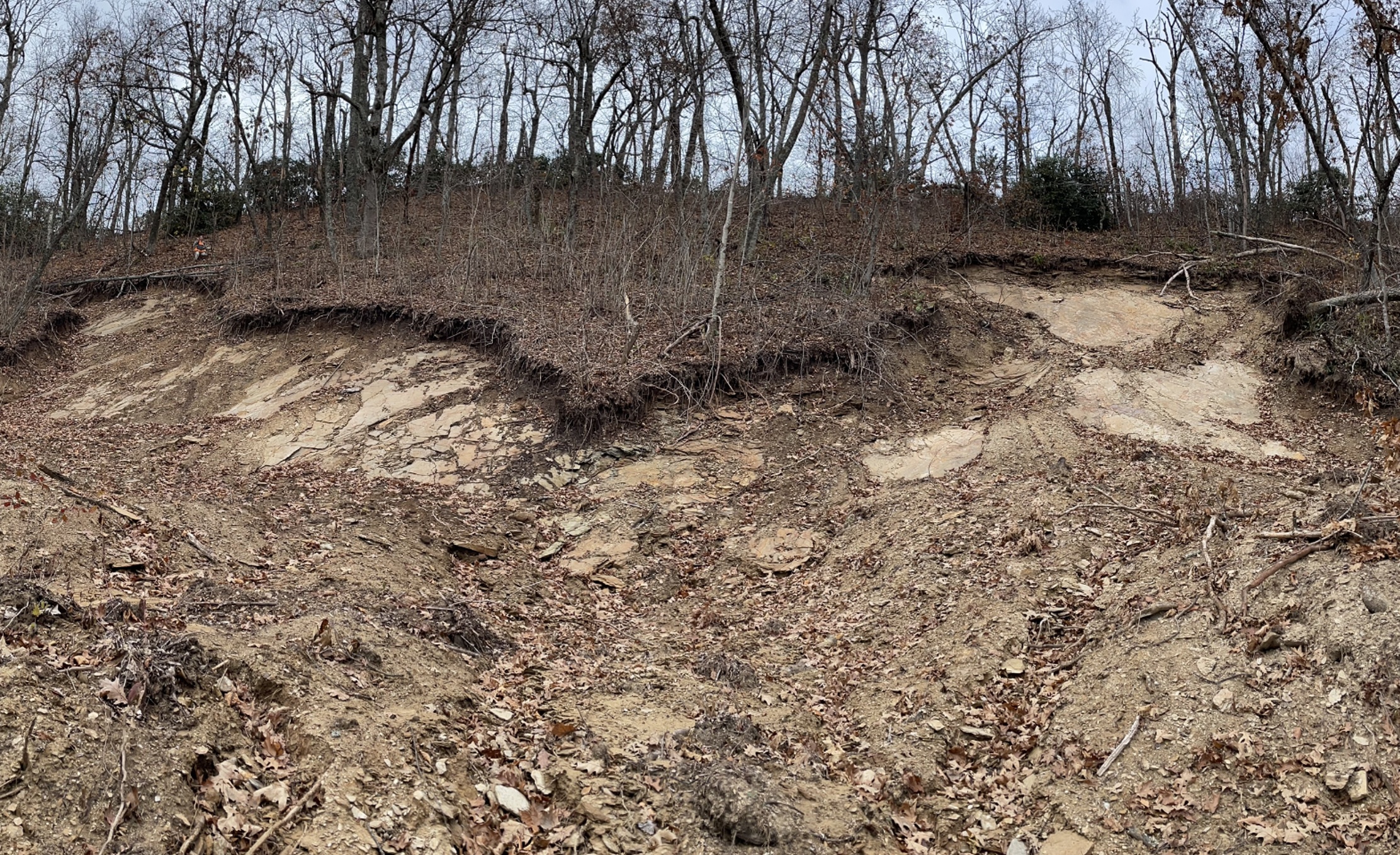
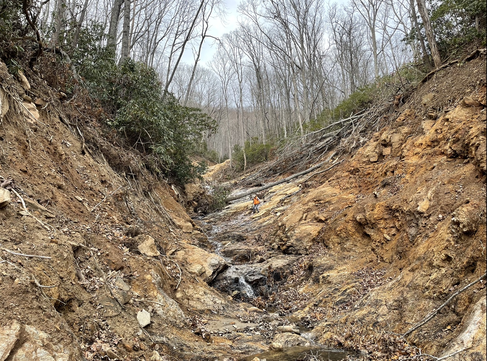
The scouring created by debris flows can be quite impressive; it greatly exceeds the potential for water erosion by small headwater streams. The picture below (taken upslope of the first photo in this post) gives an idea of what the effects of the scouring look like.
The leading edge of the debris flow contains trees and larger boulders picked up by the debris flow through its scouring action. Smaller cobbles and mud trail behind. Even small debris flows can transport surprisingly large boulders and trees due to the density of the fluidized soil (it “floats” boulders), making a debris flow strike on a structure incredibly destructive.
When debris flows exit tighter channels or ravines onto flatter ground, they often spread out, but remain mobile and destructive for some distance. In western North Carolina, many tight stream channels open onto flatter areas at the base of the steep slope. These flatter areas are older, accumulated debris flow deposits. The GIF below shows debris flows exiting a stream valley and spreading onto a flat deposit area, where buildings are destroyed. Though an unpleasant thought, this sequence of events played out many times during Helene (as well as during many other storms in our region’s history). The satellite photo below the GIF shows a bird’s eye view of the debris flow where the first photo in the post was taken.

Debris flow deposits are an indicator that an area can experience debris flows and should be developed cautiously, if at all. This often seems counterintuitive, as the flatter slopes suggest safety from landslides. In reality, these flat deposit areas are a main indicator of possible debris flow hazard. People already living in such areas should be aware of the hazard during heavy rainfall. In southern Appalachia, about 5 inches of rain over 24 hours produces conditions necessary to make debris flows possible.
This is the first post in a series of Helene-related posts discussing landslide events during the storm. Posts will be a combination of remote sensing interpretation and first-hand, on-the-ground experience. Our goal is to increase understanding of what happened during this event and help folks plan for future hazard.
Additional discussion of how debris flows fluidize can be found in this video. It’s an interesting process that isn’t fully understood, but the basics are outlined here in greater detail.
Is this the biggest boulder in the Appalachians?
by Philip S. Prince
In Pisgah National Forest a bit northwest of John’s Rock, there’s a really big boulder in the woods. Like so many Appalachian geologic features, it looks really nice when viewed with lidar imagery. This boulder is particularly satisfying to look at because it sits alone on the floor of a small valley, and its point of origin on a cliff above is quite obvious. The boulder traveled about 800 feet to its resting place, and appears to have moved alone and not as part of a larger rockslide.
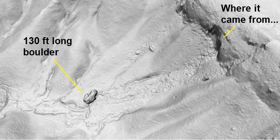
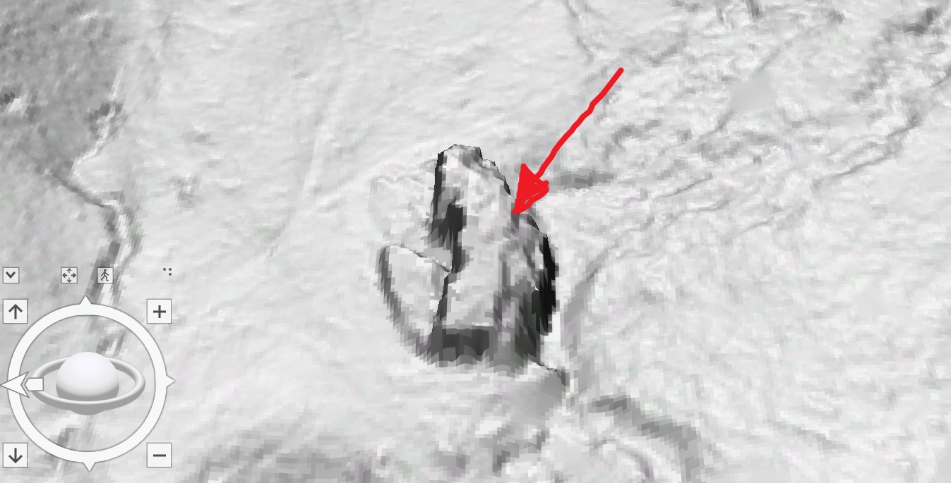
The boulder is about 130 feet long, 70 feet wide, and at least 20-30 feet thick, possibly more. It is composed of a granite-like rock, but it shows a different mineral alignment (a foliation) associated with metamorphosed rocks in the region. Despite its size, this boulder is not particularly dramatic when viewed from the ground. I tried to reproduce the ground-perspective lidar shot below during a field visit in December 2022. “A” and “B” label corresponding features of the boulder.


This boulder is actually so big that it’s hard to get a sense of its size from the ground. Enough soil has developed on parts of its surface to allow trees to grow, and the surrounding forest breaks up its outline. Adding a geologist stepping across a large crack in the boulder offers a bit of scale (lidar shot shows the crack’s location), but, ultimately, this thing is just too big to fully appreciate without a bird’s eye view.

This boulder is definitely a monster, but is it really something special within the Appalachians as a whole? I thought this was an interesting question, so I prowled a bunch of lidar in boulder-prone areas to see what I could find. Big boulders need a tough, resistant rock mass as a source, weaker rock downslope to allow them to be undercut and detached, widely-spaced fractures to permit detachment of big blocks, and enough steepness to allow them to move away from the source outcrop. These combined parameters narrow down big boulder areas, making portions of the Appalachian topographic Blue Ridge and the sandstone-capped Appalachian Plateau the best places to look. I think the southern parts of the Appalachian Plateau are better, as aggressive freeze-thaw processes during the Pleistocene likely increased fracture density to the north and reduced maximum free boulder size. The few examples below are my top contenders for biggest boulder after cruising a whole lot of lidar. I did not, of course, look everywhere, but the search produced interesting trends summed up at the end of the post.
A definite contender for Appalachia’s biggest boulder is Split Rock on the Blue Ridge Escarpment in Rutherford County, North Carolina (it’s on private property and can’t be freely accessed). Split Rock is about 150 feet long in its longest dimension, though splitting into three pieces has allowed it to spread a bit. Its proportions are actually quite comparable to the Pisgah boulder and are probably just about identical if Split Rock were “un-split” and reassembled.
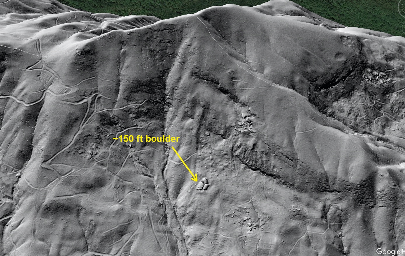
Like the Pisgah boulder, Split Rock is too big to really appreciate from the ground and could be easily confused for in-place bedrock outcrop. The photo below shows the edge of Split Rock at one of the namesake splits; the lidar shot shows the photo location.


Split Rock is composed of metamorphic gneiss-like bedrock that is distinct from the granite-like rock of the Pisgah Boulder. Split Rock’s most impressive detail is that it did not completely fall apart on its trip downslope, as the rock is full of weaker mica-rich horizons along which it might break apart. Its variable compositional layering (which is a metamorphic foliation) gives it the ragged edges visible in the field photo above.
Several boulders in the 100 foot size range occur within Split Rock’s part of the Blue Ridge Escarpment, but the most prolific giant boulder province in southern Appalachia–and likely all of Appalachia–is the western edge of the Cumberland Plateau in Tennessee and Kentucky. Here, thick sandstone layers undamaged by thrust faulting and folding are well-suited to forming giant boulders. Folded and faulted layers in the Valley and Ridge contain too many fractures to make bigger boulders than the Plateau sandstones, and mica content and general weatherability in the Blue Ridge limit huge boulder potential outside of isolated extreme examples.
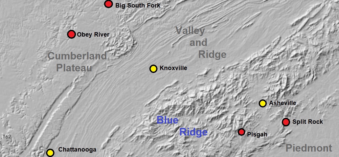
The slope above the Obey River shown below is a good example. The boulders looks small, but they are actually just shy of the size of the Pisgah boulder. Boulders this size are actually very common in this area, where soluble limestone beneath the sandstone caprock and a history of river incision set the stage for moving huge blocks downslope. The boulders shown below traveled as part of a larger landslide, but give the appearance of having moved independent of one another after the initial failure of the cliff line.
To the northeast, on the Big South Fork River near the Kentucky border, two large sandstone boulders detached from a cliff outcrop and plowed a clearly visible path downslope toward the river. the largest boulder, closest to the river, is about 115 feet long in its longest dimension.

A friend provide me with a photo of the 115 ft boulder, taken right at the end of the yellow leader line in the image above. Notably, these big sandstone boulders are not deeply buried in soil like the Pisgah boulder and Split Rock.

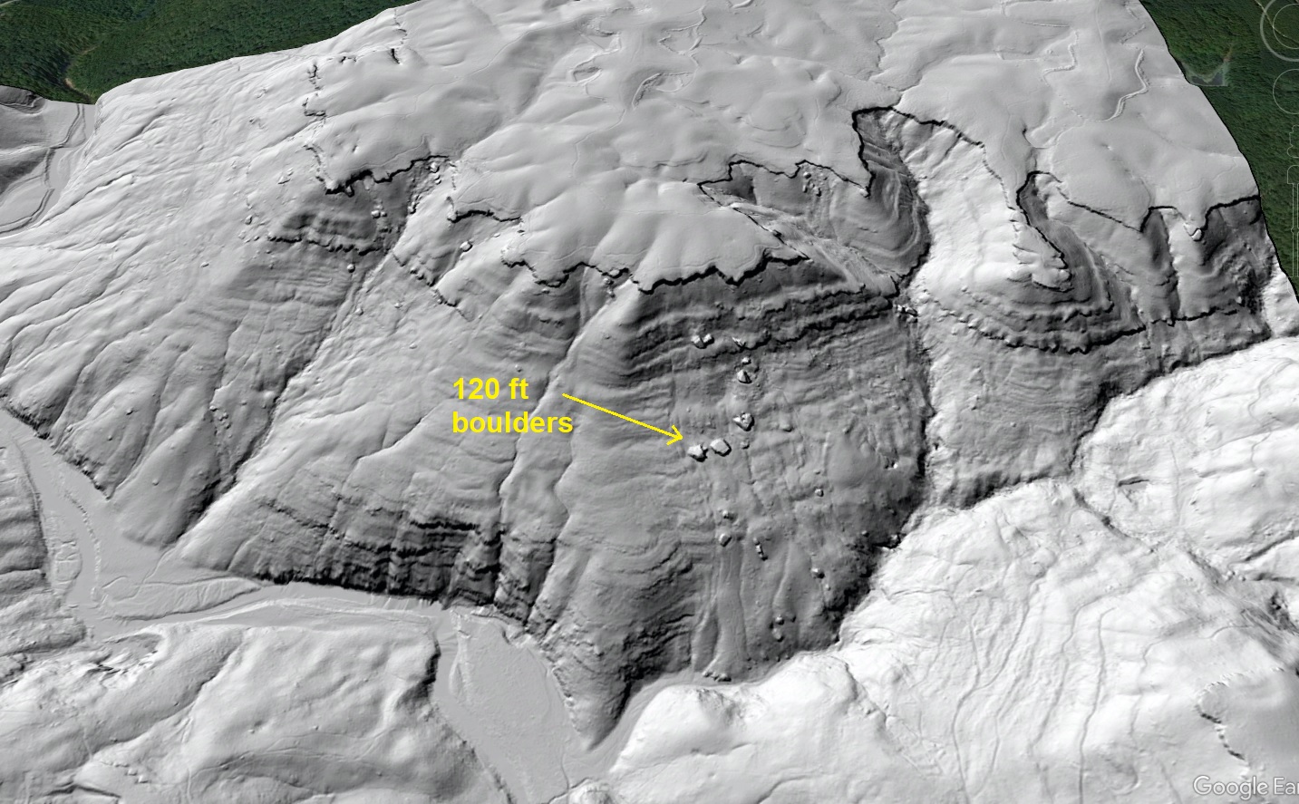
Further north in Kentucky, the Red River Gorge area is also full of ~120 foot sandstone boulders. The lidar shot below (taken from the Kentucky Geological Survey’s site) shows two 120-footers, indicated by red arrows. Boulders between 50 and 100 feet along their longest dimension are extremely common in this area. The joint-controlled, right-angle patterns in the cliff lines in this area are also interesting to check out.

The zoomed-in shot below shows the lower right boulder, which has traveled about 400 feet from the cliffline.

If you’ve paid attention to the measurements, 120 feet or so seems to be a common measurement for the biggest boulders to be seen in boulder-prone Appalachian landscapes. The Pisgah boulder and Split Rock aren’t alone in the southern Blue Ridge area; there are more 100-120 ft boulders to be found there, but they aren’t as numerous as boulders of that size in the Appalachian Plateau. In both areas, though, maximum size is intriguingly consistent, though only among boulders that have moved several boulder lengths from their source outcrops. Bigger chunks of rock can be found right along cliff lines, but these detached blocks have not actually moved or slid and experienced the associated physical forces. I imagine that the ~120 ft number is some reflection of the physical properties of the boulder-forming rock unit, both in terms of how it resists falling apart during sliding and how it controls topography to make cliffs and slopes to source and move big boulders. The image below compares sizes of the some of the boulders, with zoom adjusted so that it’s possible to directly compare them.

So, is the Pisgah boulder unique in any way? I think so. It is definitely at the top end of boulder size within Appalachia, though you can’t justifiably conclude it’s bigger than a reassembled Split Rock or something lurking in the Cumberland Plateau. It also traveled a significant distance from its source outcrop. This is notable because it contains aligned mica-rich layers that present plains of weakness along which it could break apart. The fact that the Pisgah boulder (and Split Rock) traveled hundreds of feet at their significant sizes and ended up in (mostly) one piece is impressive and probably the result of some amount of coincidence. Thick-bedded, very quartz-rich sandstone boulders lack aligned mica layers, so the potential to move a single huge piece of rock without breakup might be greater.
I don’t know how mechanical properties of the respective rock types would compare. Tensile strength of all Earth rocks is quite low compared to compressive strength, so rock doesn’t do well when forces try to pull it apart. Mica-rich zones or zones of extreme mineral weathering might lower tensile strength even more, so non-sandstone rocks might be less likely to hold together in single chunks than a physically hard and chemically tough quartz-rich sandstone. I also don’t know how these boulders move. I have always assumed that they slide, as tumbling would subject them to forces that would break them down to smaller pieces (that whole tensile strength thing, again). Check out what happens to the big block of rock in Switzerland shown below at this link.

Ultimately, geology superlatives (biggest, oldest, etc.) aren’t really worth much, but trends and patterns are useful in understanding how landscapes work. I looked at hundreds of big boulders, and not too much over 100 feet in the longest dimension is as big as you’ll see for a boulder that has moved significantly. This size is well-represented in certain sandstone-rich areas. Notably, sandstone-capped areas in Kentucky and Tennessee have, on average, bigger boulders than sandstone-capped portions of West Virginia. This may reflect local geologic details, climate and latitude, or both. The Blue Ridge serves up arguably the biggest boulders, though by an insignificant margin, and they are much less numerous due (presumably) to rock type details. Perhaps most interesting is that no one has ever seen a boulder the size of these biggies actually moving in the Appalachians, and none of them appear to be freshly emplaced. What makes them move and whether or not they do much moving under modern-day climate conditions is a big question in and of itself.
Using LiDAR and a 121-year-old drawing to locate a 1901 debris flow in North Carolina’s Blue Ridge Mountains
Philip S. Prince
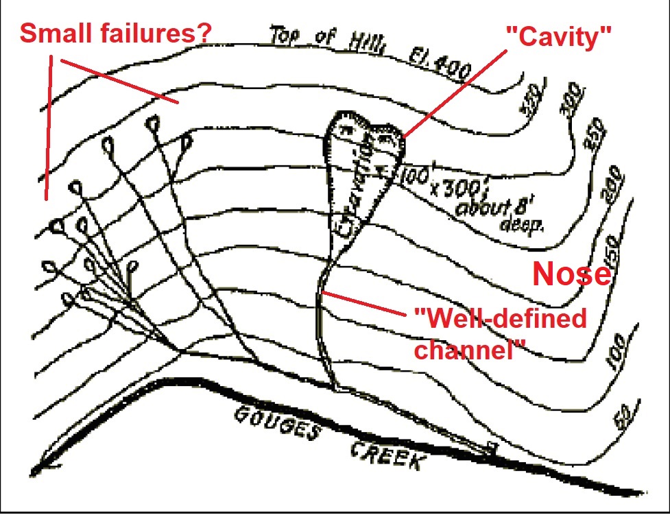
In 1902, E.W. Myers published an account of a 1901 flood (the “May Fresh”) and its effects on the mountain landscapes of western North Carolina. Included in the report is the following sketch of a debris flow, sourced in digital form from Anne Witt’s ResearchGate page. Notably, no indication of cardinal directions or distance to nearby landmarks are included in the sketch, making the exact location of the debris flow (whose indicated size is impressive!) uncertain.

Also excerpted in Anne’s work is Myers’ text description of the feature he drew.

I thought it would be interesting to try to find this debris flow based on the information Myers provides. With the sketch and text, Myers indicates that the debris flow entered Gouges Creek from a downstream-left direction, left a “heart-shaped” scar on the hillside, and was near a ridgeline and summit and generally very high within the surrounding landscape. In the era of high-resolution LiDAR imagery, these details turned out to be sufficient to locate the debris flow on the Mitchell County-Avery County line north of Spruce Pine, North Carolina. A LiDAR hillshade image of the slide, as well as a Google Maps image of its location, are shown below. The slide is not large in the context of the entire mountainside, but the heart-shaped scar from the initial failure (end of yellow arrow), downslope scouring, and proximity to the ridgecrest/summit are clearly visible.


Locating the debris flow was easier than expected. It is the only significant debris flow on Gouges Creek (not to be confused with Gouge Creek and many other Gouge place names in Mitchell County), and its distinct heart-shaped initiation zone distinguishes it from other debris flow features on nearby slopes. A close look at the “heart shaped” scar as revealed by LiDAR hillshade makes clear what Myers hoped to capture with his sketch.

A 2023 geologist of the Google Earth and drone era has to remember that Myers drew his 1901 or 1902 map sketch by interpreting from the ground, and he was quite successful in capturing the general layout of the landscape around the debris flow. No indication of his vantage point for making his sketch is given in the drawing of the text excerpt; he may have been along Gouges Creek or viewing from the ridge to the south. The images below compare the actual topography to Myers’ sketch, with labels on notable features. The light blue lines in the LiDAR image indicate faint channels with may generally locate the many small failure Myers illustrated. No significant trace of these failures is visible in today’s landscape.

Myers did overestimate the size of the failed area, but he didn’t do badly assuming he was visually estimating from a distance. The actual scar is a bit smaller than he suggested, but is still quite significant. The LiDAR detail below shows the real dimensions of the scar, assuming Myers length estimate was made from the top of the “heart” to where the failed area narrows to the scoured channel.

Myers also reported that the material which moved during the debris flow seemed to have “disappeared utterly,” indicating that the flow was quite mobile and did not deposit significant material in Gouges Creek near the failure itself. This observation is reflected in LiDAR imagery, where no significant deposit is visible in the area shown; instead, scouring continues down the Gouges Creek channel. The yellow arrow indicates the heart-shaped initiation zone.

Myers did not use the term “debris flow” (I don’t think it existed at the time!), but his description captured some principal components of debris flows, included the “excavated” initiation zone (“evacuated” would be used today), erosion or scouring of a track into the soil profile below the initiation zone, and the high mobility of the moving material. The simple physical model below shows this scouring process, during which the once-solid material that detached to produce the debris flow fluidizes and erodes the slope as it travels downhill. Compare the pre-flow “normal” channel texture to the post-flow scour. This erosion adds material to the flow, making it grow in volume. A key distinction between the model and a real debris flow is that the model uses dry, low friction materials; a real debris is a very “wet” feature that occurs due to soil saturation as a result of extreme rainfall.

LiDAR reveals other past debris flows in the area, including an impressive feature (left arrow, below) northwest of the Gouges Creek flow. The GIF shows the outline of the flow and its path from the initiation zone downslope.

This debris flow has a less impressive scar/initiation zone, but the flow did leave traces of a process known as “superelevation,” which describes a flow sloshing up the sides of bends in the channel carrying it due to its momentum.

The GIF below shows another physical model, which demonstrates superelevation. Note how the flow runs up the channel banks where bends are present.

I haven’t read the full Myers report, so I don’t know if the superelevating debris flow is discussed or if it is even from the 1901 “May Fresh”–there are plenty of other extreme precipitation events to choose from. In any case, the physical characteristics of the superelevating flow are sufficiently distinct from the Gouges Creek debris flow to distinguish them with LiDAR imagery with the help of Myers’ sketch and description.
The scar and track of the Gouges Creek debris flow are now located in an entirely forested landscape, and would be visible only from the ground due to tree cover. With LiDAR imagery, however, the feature is impressively visible and fresh-looking despite being 116 years old at the time of LiDAR data collection.

The Gouges Creek debris flow did destroy a log cabin; apparently it was unoccupied or uninhabited, and no one was hurt or killed. While modern land use patterns are different in the North Carolina Mountains, debris flows still represent a significant threat to life and property due to their extreme mobility and fast speed (you can’t outrun one). Were a debris on the scale of the Gouges Creek event to occur in a more populated part of the mountains today, the potential for very negative outcomes is quite high. Mountain residents need to be aware of the weather conditions that produce debris flows, as well as their potential paths, to stay out of harm’s way. Records of past events like Myers’ report are useful reminders of the potential for extreme rainfall and debris flows throughout the North Carolina Mountains, though events may be separated by years or decades in a given area.
Did humans cause this Alleghany County, Virginia, mountaintop to drop several feet?
by Philip S. Prince
*Note: There is indeed a sand model in this post, but it’s near the end…
Well, it’s more of a hilltop, but it has dropped several feet since iron mining was active on its lower slopes in the early 20th century! The summit of this unnamed hill southwest of Low Moor, Virginia, hosts conspicuous scarps that define a graben, or downthrown block, that has sunk about 6 ft (just under 2 m) relative to the surrounding hilltop. The graben is a bit over 300 ft (100 m) wide. The scarps are subtle but very clearly visible in 1-meter resolution, lidar-derived hillshade imagery. Results of iron mining are visible at lower right in the upper image below (more on this later, for sure).


The scarps (which face outwards and downhill) and counter-scarps (which face inward, or towards the upslope direction) do not appear to cut road grades on the slope. They do, however, offset a prospect trench within the subsided graben. The slope movement thus post-dates the trench, but was likely gradual and episodic over the course of months or years. I don’t know if movement would have been discernible during the period that mining was active, or if it completely post-dates work at the site.

Disturbance of the prospect trench puts movement on the scarps within, or after, the iron mining period, which is consistent with other iron-mine related features in Alleghany and Botetourt Counties in Virginia. I have written about these other iron mine-related landslides before (click here), but the summit graben shown here is unique because of its position on the slope and its 300 ft / 100 m width relative to the overall scale of the affected hill. Because of the graben’s position on the hill and its width, deformation is likely seated very deep within the hill. The slow-moving GIF below shows an interpretive cutaway of the slope, with shear planes sketched in from the shape of the slope and reasonable angular relationships.
Interpretive is the key word here…I have not even been to this site in person, so I am just inferring a possible subsurface structure from surface deformation and the size and shape of the hill and graben. That said, the graben is quite large with respect to the size of the hill, and its position so far from the toe of the slope definitely implies very deep-seated movement. This is certainly not a thin, translational bedrock-involved slide of the type that is common within the Appalachian Valley and Ridge. The outwardly-moving hillslope is not a dip slope in the first place, and the scale and position of the graben make a shallow translational explanation impossible. A slightly zoomed version of the subsurface interpretation is shown below. Note that the cut of the diagram is a bit out of plane of the oblique image and slightly exaggerates relief and the thickness of the moving area.

Where does the iron mining factor into the story? Highwall surface mining for limonite ores occurred along the foot of the hill in the early 20th century. The workings were not exceptionally large, but they did tend to make contour-parallel cuts along the foot of the slope. The largest of these (the one visible at lower right in the post’s first image) appears to have experienced a major collapse. The other cuts also show indication of slope movement, though it is less pronounced. Mined areas and their location with respect to the graben are shown below.

Even though the mined areas aren’t exceptionally extensive, they obviously destabilized the slope in proximity to the cuts; small parallel scarps are visible upslope of the mined areas in the image above. Presumably, this destabilization and associated slope movement turned out to be very far-reaching, allowing the whole hill to expand a bit laterally and force graben subsidence. The following GIF offers a simplified, cartoon-style interpretation of the process.

This style of slope movement suggests that hillslopes in the area may be near a deep-seated stability threshold that makes them susceptible to modest but volumetrically significant movement in response to very minor surface modification. This susceptibility may be a reflection of bedrock geology and structure. This area is underlain by a complexly folded and faulted sandstone and limestone interval with thick shales above and below. The result is shale-cored mountain topography that is “propped up” by the strength of armoring sandstones. Additionally, the area has experienced considerable geologically-recent relief production due to its location in the James River basin, so slopes have grown taller and steeper as valleys have lowered. Given these background conditions, potential slope behavior under disturbance could be expected to be different from the behavior of a more geologically consistent, lower relief landscape.
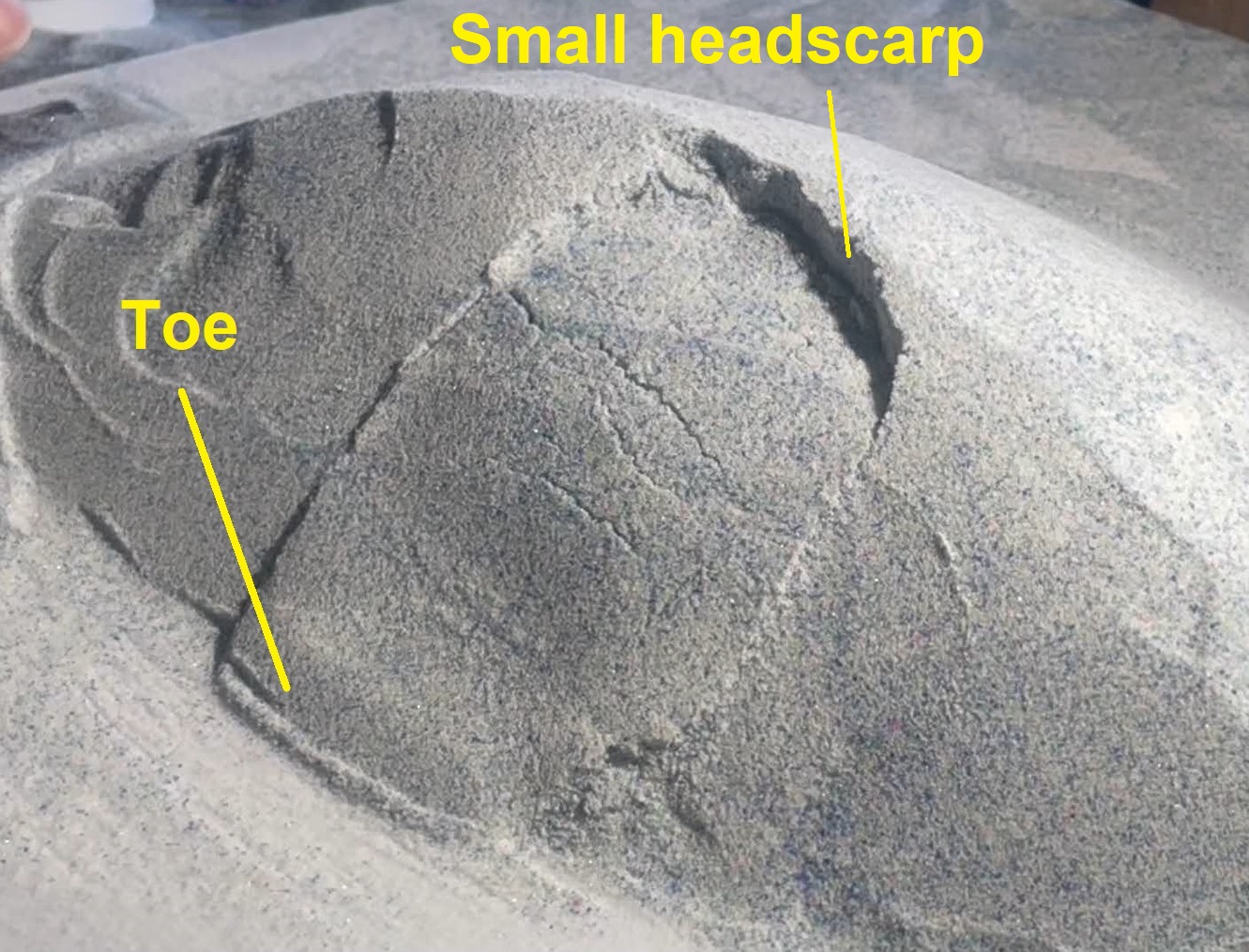
I think the most interesting aspect of this human-induced topographic “adjustment” is how a very modest excavation produced an equally modest slope movement, at least in terms of overall displacement of the moving mass of hillslope. None of the mining-related slope movements in the area appear to have produced rapid, long-runout slides or flows; all resulted in slight shifts that are really only discernible with lidar-derived imagery. All are reforested, and lidar imagery does not suggest any are subject to imminent significant movement. I tried to set up a simple physical model to capture this behavior. Two trials are shown below. The model hillslope is constructed of a cohesive sand-and-flour “shell” over a weak glass microbead core. With disturbance of the toe of the slope, a small, lurching failure occurs, reestablishing equilibrium and stability with a tiny but obvious movement.

Setting these models up to produce this style of failure was a worthy challenge. Their behavior is definitely material-specific; cohesive or loose sand alone (or microbeads) won’t do it. The slope has to be just unstable enough–and mechanically appropriate–to settle slightly with minor disturbance to the toe of the slope. The failures are not as deep-seated with respect to the slope as the real graben scenario, but they are deep enough to produce back rotation of the head of the slide with very little displacement, as shown below. Scarps and counterscarps are marked with hachured lines.

While these models experience rapid, one-time movement, the amount of movement necessary to reestablish stability is very small. This was the goal of the models, specifically as a way of connecting the slope’s mechanical architecture to failure behavior. A very brief YouTube video linked below shows the actual failures at full speed. It seems ridiculous to go to great lengths for such tiny movement, but it was much more challenging than producing a high-runout model, for sure.
While the summit graben feature is an extreme example, mine-related failures abound in this area. The image below shows other failures just up the valley from the graben feature. Again, cuts on contour appear to be the issue, but slopes responded with modest movement. In the image below, a large area of slight displacement is clearly visible above a highwall cut. The hill with the graben is just outside the field of view to the right. More examples exist just southwest of this one.

The location of these slope has largely spared them from modern-day engineering, but it is interesting to consider how they might respond to more carefully planned modification! It also invites comparison to the well-documented Rattlesnake Ridge landslide in Washington.
Scale model landslides show what happens if you mess with a landslide toe
by Philip S. Prince
The two images below show the same model landslide at different points during its evolution. The lower image, of course, looks much uglier, with a broken-up slide block and huge, looming headscarp. Notably, the thick toe labeled in the upper image is conspicuously missing…(spoiler: you can watch this model evolve at 1:04 in the video link at the end).
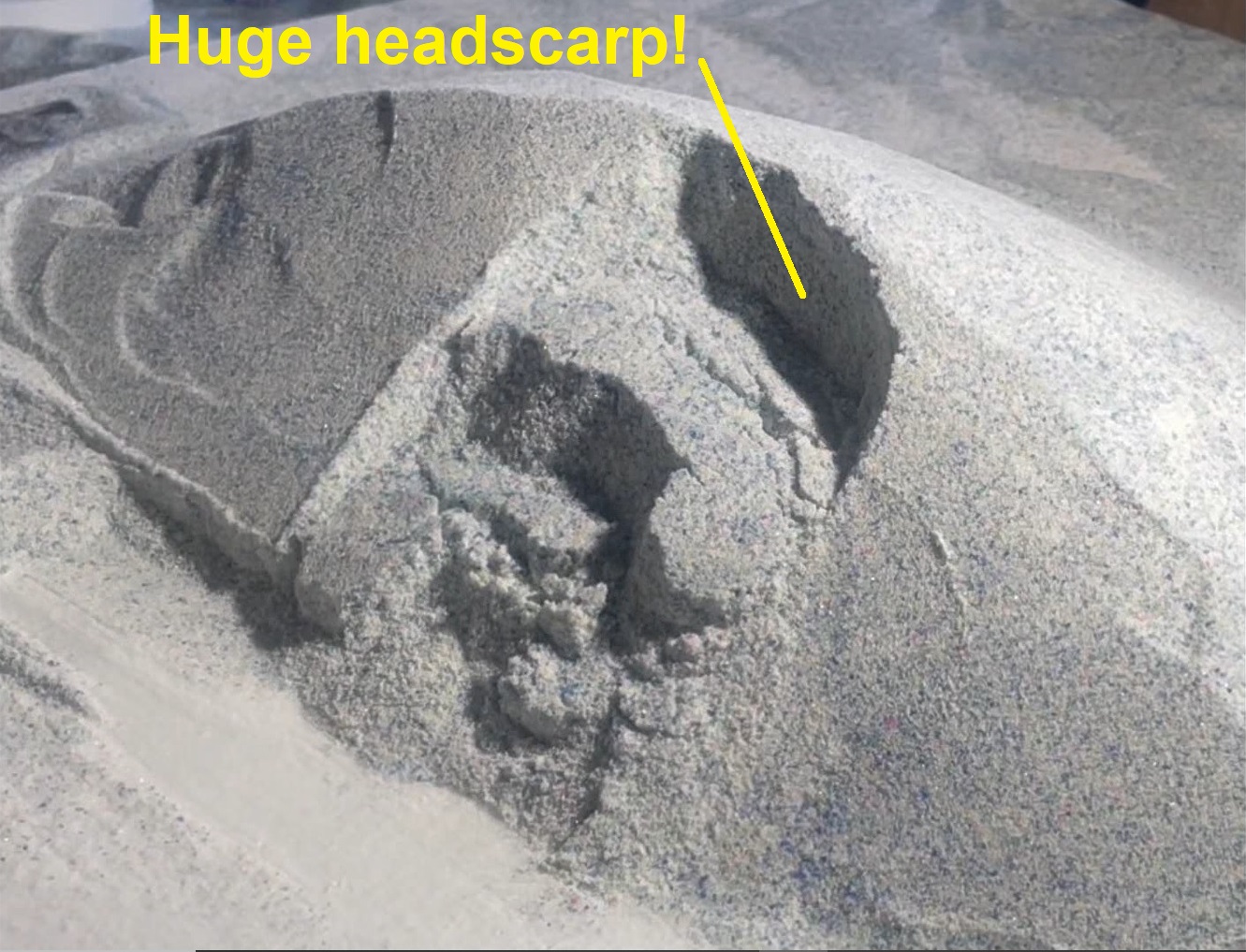
So, how did the slide progress from a not-too-impressive feature to a mangled mess? The answer relates to that toe, or rather its absence in the lower image, with a few details of the slide’s shape thrown in (more on that in a bit). Toe removal, however, is the main idea, and removing a landslide’s toe invites trouble in the form of probable continued movement. A slide like the one shown above (that is, not a rapid, flow-type slide) can move until the toe becomes large enough to resist the driving load that led to slide movement, assuming that friction on the sliding surface remains low. Removing the toe allows driving load to overwhelm resistance again if friction on the slide plane is sufficiently low, leading to renewed movement of the slide. The GIF below illustrates this idea in basic terms. I-26 drivers in western North Carolina might appreciate the pink excavator…

A well-developed landslide toe can therefore be regarded as the “prop” that supports the rest of the upslope slide mass atop the weak failure surface. Altering a toe is often a fast track to instability and slide reactivation. The simple model shown in the GIF below demonstrates toe development, removal, and reactivation in a slide that behaves much like the one drawn above. When toe material is removed, the slide advances until enough supporting toe is restored. Note that this model is much “neater” than the model in the first images!

Continued toe removal leads to continued motion, particularly in the model above, as the slide mass does not break apart and continues to exert a strong driving load on its base. Once the slide mass is broken along its edges (lateral scarps), it no longer has the small amount of support provided by the cohesion (“stickiness”) of the model material. Real rock and many soils have some cohesive strength as well. It is never very much, but it does provide a component of resistance to sliding. Once the material is broken, however, this tiny bit of resistance is lost, and ongoing movement of the slide due to toe removal is that much easier. In a model like the one above, the entire slide block can be consumed by removing the initial toe and continuing to remove material pushed out into the new toe.
Weakness and potential instability associated with a landslide can persist for a long time after the slide becomes dormant and is not obvious in the landscape. Nearly “invisible” old slides that aren’t currently moving can be reactivated long after they stopped moving by disturbing the slide toe. Using lidar to identify such old slides is a key part of pre-construction site assessment.
Destabilization of landslides by toe removal is a very real thing, with actual scenarios–both large and small–arising from construction and natural stream or wave erosion. Many are slow and manageable, but they can be ongoing, hard to stop, and quite expensive over time. A famous example I am fond of is shown below. This is the “Galloping Highway” slide in Giles County, Virginia, along US 460. The toe of an older, dormant slide was removed for the highway cut, initiating literally decades of reactivated–and slowly ongoing–movement. This slide is, in effect, a real-world example of the previous GIF where an “invisible” slide came back to life. The slide block is nearly 1,000 feet across along US 460.

The slides shown below are in McDowell County, North Carolina. Both are situated for possible reactivation due to the road cut that has impacted their toes as well as steady stream erosion of the toes, which would pre-date the road cut. I imagine both have a reactivation history due to stream erosion; the smaller slide on the right appears to have reactivated more recently due to the road cut.

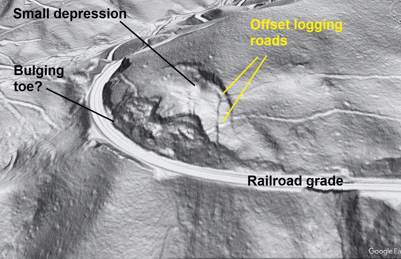
The next impressive example is along a railroad grade in western North Carolina. Lumpy areas just above the tracks look very much like recent reactivation, and a faint toe seems to be pushing out of the base of the cut. Two logging roads at the right of the slide are offset by scarps, indicating recent slide movement. The relative impact of the railroad cut and possible removal of material from the slide toe as it slowly pushes outward can’t be discerned from lidar, but the offset roads and ugly toe indicate this one definitely deserves engineering attention.
The slide above looks quite different from the first few examples and provides a nice way to circle back to the very first model in this post. The shape of a landslide’s failure (sliding) surface strongly impact what happens to the sliding mass as it moves downhill. A slide on a failure plane with constant slope can move intact, but a failure plane with changing slope requires the slide mass to constantly change its shape as it moves. If the failure plane becomes less steep, the top of the slide has to stretch to match its shape, forcing cracks or new internal scarps to form. The uppermost part of the slide can actually tilt backward until a depression forms (see above and below). The more the slide moves, the more exaggerated the cracking, internal breakup, and back-rotation of the upper part of the slide become. The GIF below illustrates the initial phases of the concept.
Obviously the gap below the slide block can’t exist…the collapse and stretching of the block are constantly developing as it moves. Physical models offer a nice way to show this process in action. Note how the cracking accompanies the backwards tilting of the upper part of the slide. This model is the last one shown in the video link.

So what happens to these early cracks if the toe is removed and movement continues? With the right failure surface shape, something like the very first model develops. This is where the video comes in. Linked below are more reactivated landslide models, including all those shown above. Some really fall apart with toe removal and continued movement; in others, a smaller and smaller block continues downslope with little or no internal break-up. I assure you that this is the ONLY place you will see this many model landslides in one place, whatever that may mean! The two styles of slide described in this post are represented. They can be distinguished by how much the slides break apart as they continue to move after toe removal. I think it’s cool to watch their motion all at once. It beats trying to piece together months or years of episodic movement!
