by Philip S. Prince
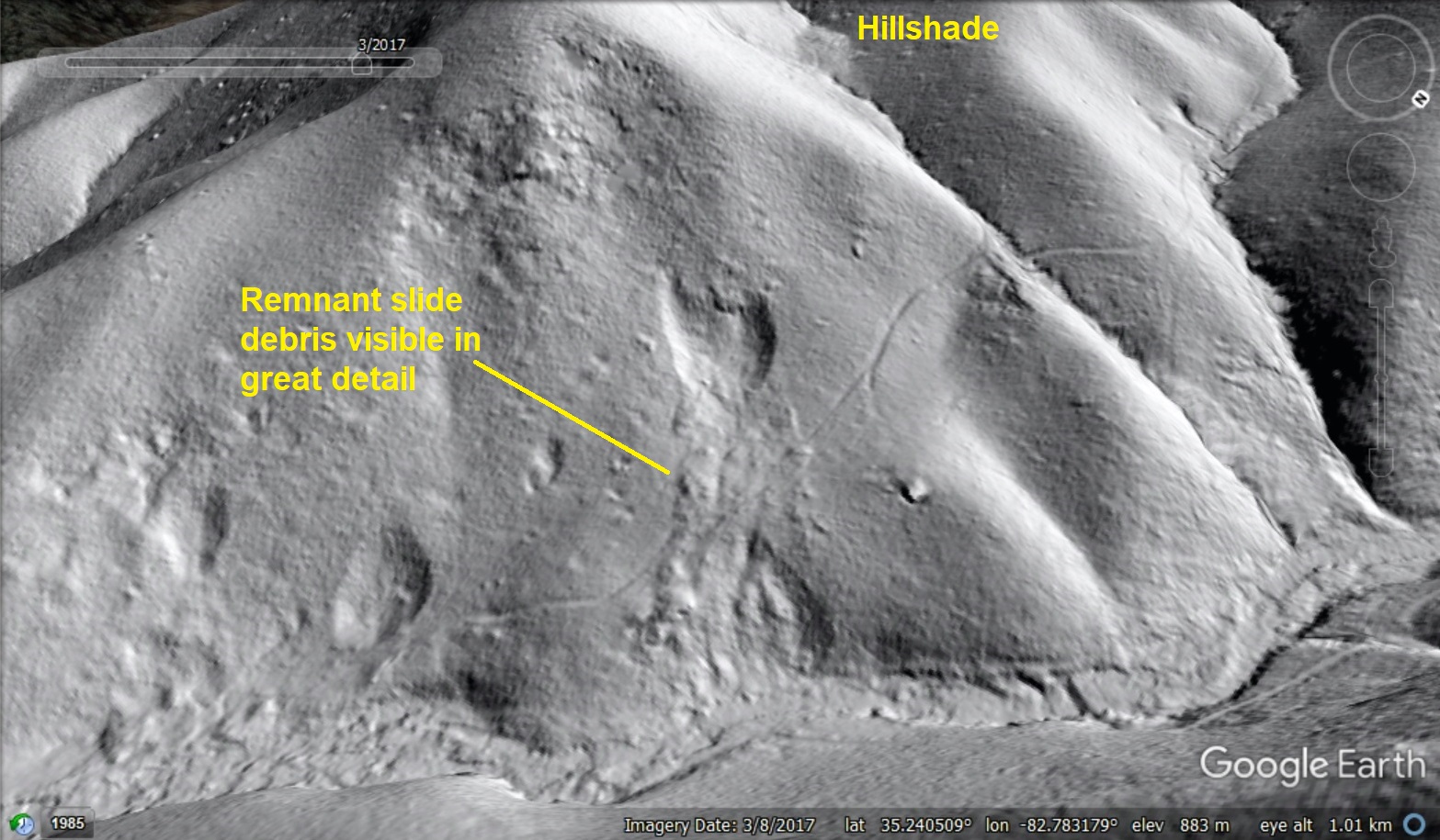
In Pisgah National Forest a bit northwest of John’s Rock, there’s a really big boulder in the woods. Like so many Appalachian geologic features, it looks really nice when viewed with lidar imagery. This boulder is particularly satisfying to look at because it sits alone on the floor of a small valley, and its point of origin on a cliff above is quite obvious. The boulder traveled about 800 feet to its resting place, and appears to have moved alone and not as part of a larger rockslide.
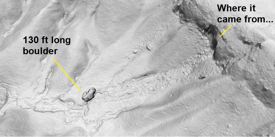
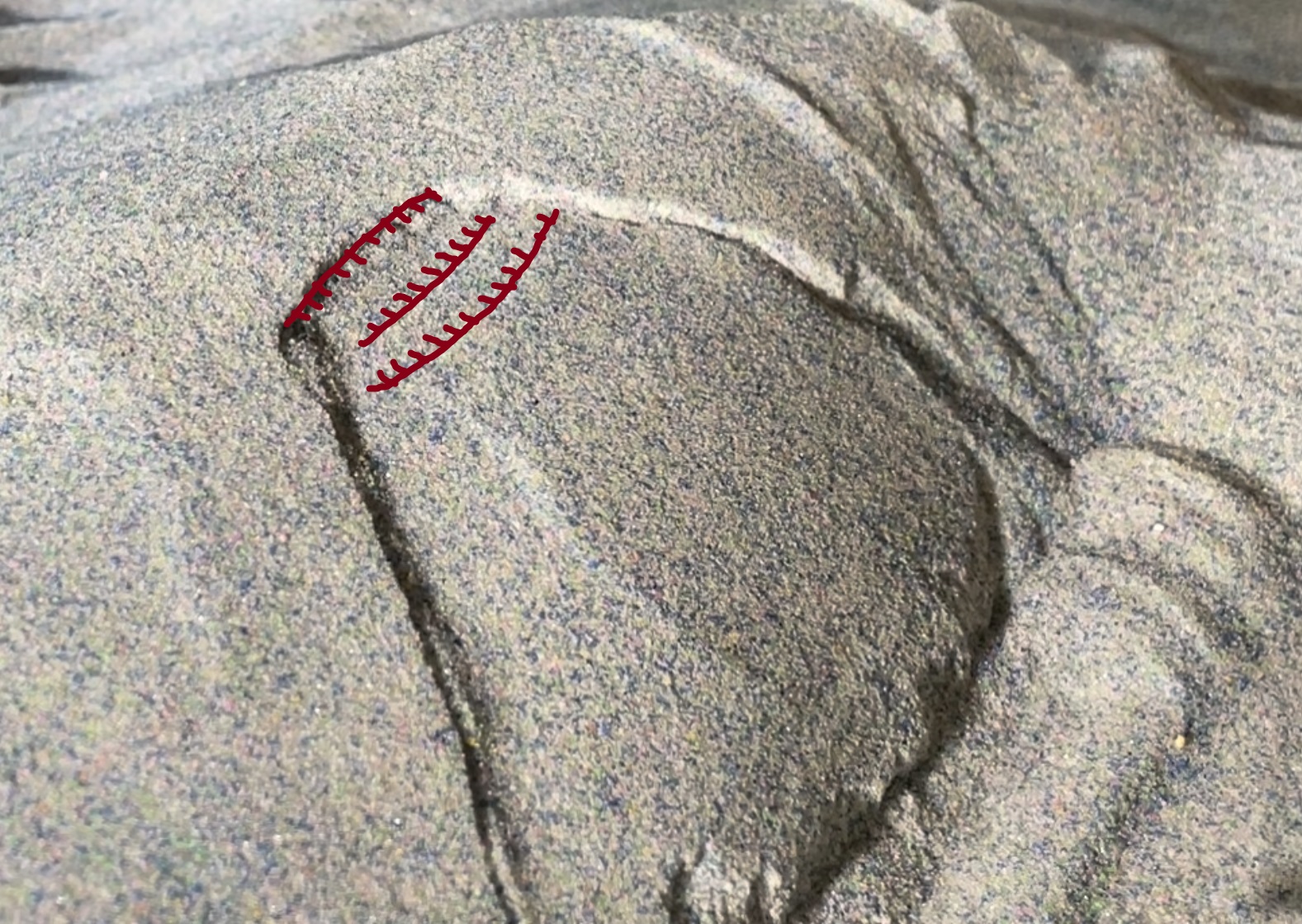
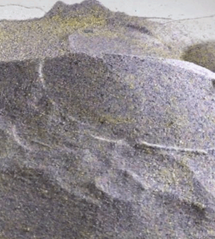
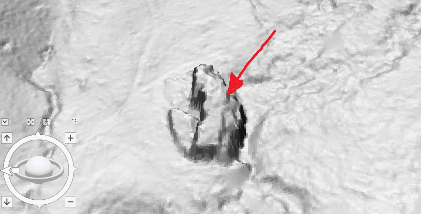
The boulder is about 130 feet long, 70 feet wide, and at least 20-30 feet thick, possibly more. It is composed of a granite-like rock, but it shows a different mineral alignment (a foliation) associated with metamorphosed rocks in the region. Despite its size, this boulder is not particularly dramatic when viewed from the ground. I tried to reproduce the ground-perspective lidar shot below during a field visit in December 2022. “A” and “B” label corresponding features of the boulder.


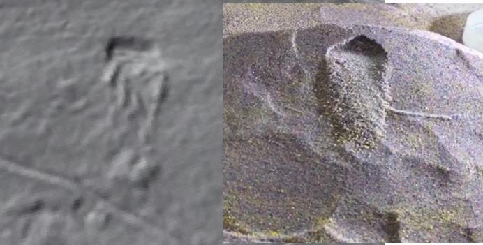
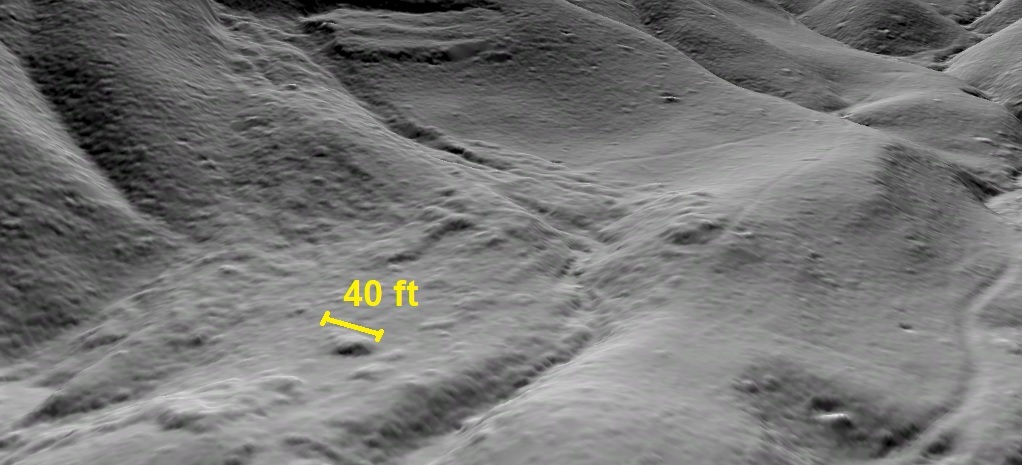
This boulder is actually so big that it’s hard to get a sense of its size from the ground. Enough soil has developed on parts of its surface to allow trees to grow, and the surrounding forest breaks up its outline. Adding a geologist stepping across a large crack in the boulder offers a bit of scale (lidar shot shows the crack’s location), but, ultimately, this thing is just too big to fully appreciate without a bird’s eye view.

This boulder is definitely a monster, but is it really something special within the Appalachians as a whole? I thought this was an interesting question, so I prowled a bunch of lidar in boulder-prone areas to see what I could find. Big boulders need a tough, resistant rock mass as a source, weaker rock downslope to allow them to be undercut and detached, widely-spaced fractures to permit detachment of big blocks, and enough steepness to allow them to move away from the source outcrop. These combined parameters narrow down big boulder areas, making portions of the Appalachian topographic Blue Ridge and the sandstone-capped Appalachian Plateau the best places to look. I think the southern parts of the Appalachian Plateau are better, as aggressive freeze-thaw processes during the Pleistocene likely increased fracture density to the north and reduced maximum free boulder size. The few examples below are my top contenders for biggest boulder after cruising a whole lot of lidar. I did not, of course, look everywhere, but the search produced interesting trends summed up at the end of the post.
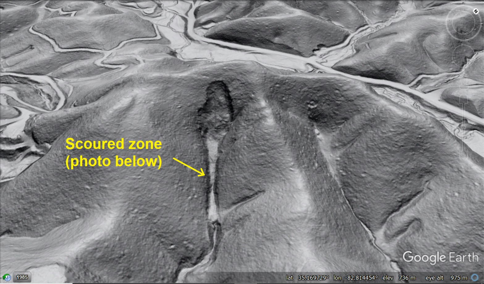
A definite contender for Appalachia’s biggest boulder is Split Rock on the Blue Ridge Escarpment in Rutherford County, North Carolina (it’s on private property and can’t be freely accessed). Split Rock is about 150 feet long in its longest dimension, though splitting into three pieces has allowed it to spread a bit. Its proportions are actually quite comparable to the Pisgah boulder and are probably just about identical if Split Rock were “un-split” and reassembled.
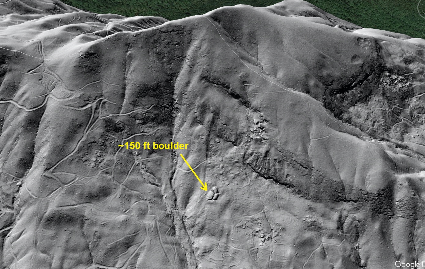
Like the Pisgah boulder, Split Rock is too big to really appreciate from the ground and could be easily confused for in-place bedrock outcrop. The photo below shows the edge of Split Rock at one of the namesake splits; the lidar shot shows the photo location.


Split Rock is composed of metamorphic gneiss-like bedrock that is distinct from the granite-like rock of the Pisgah Boulder. Split Rock’s most impressive detail is that it did not completely fall apart on its trip downslope, as the rock is full of weaker mica-rich horizons along which it might break apart. Its variable compositional layering (which is a metamorphic foliation) gives it the ragged edges visible in the field photo above.
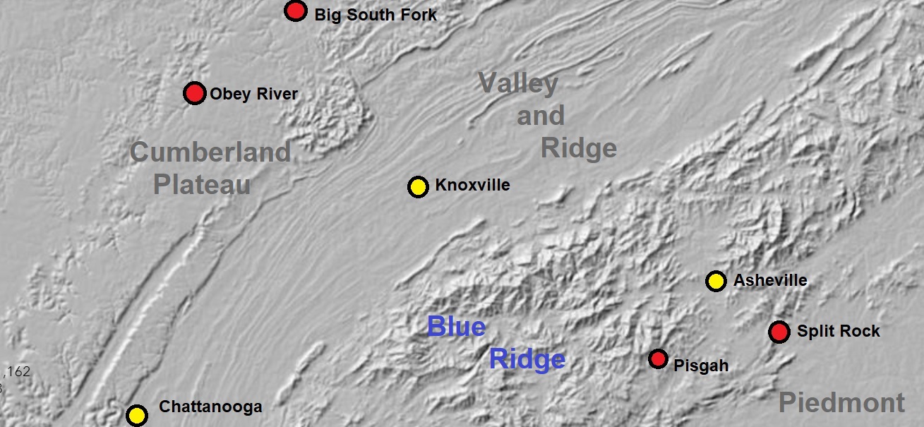
Several boulders in the 100 foot size range occur within Split Rock’s part of the Blue Ridge Escarpment, but the most prolific giant boulder province in southern Appalachia–and likely all of Appalachia–is the western edge of the Cumberland Plateau in Tennessee and Kentucky. Here, thick sandstone layers undamaged by thrust faulting and folding are well-suited to forming giant boulders. Folded and faulted layers in the Valley and Ridge contain too many fractures to make bigger boulders than the Plateau sandstones, and mica content and general weatherability in the Blue Ridge limit huge boulder potential outside of isolated extreme examples.
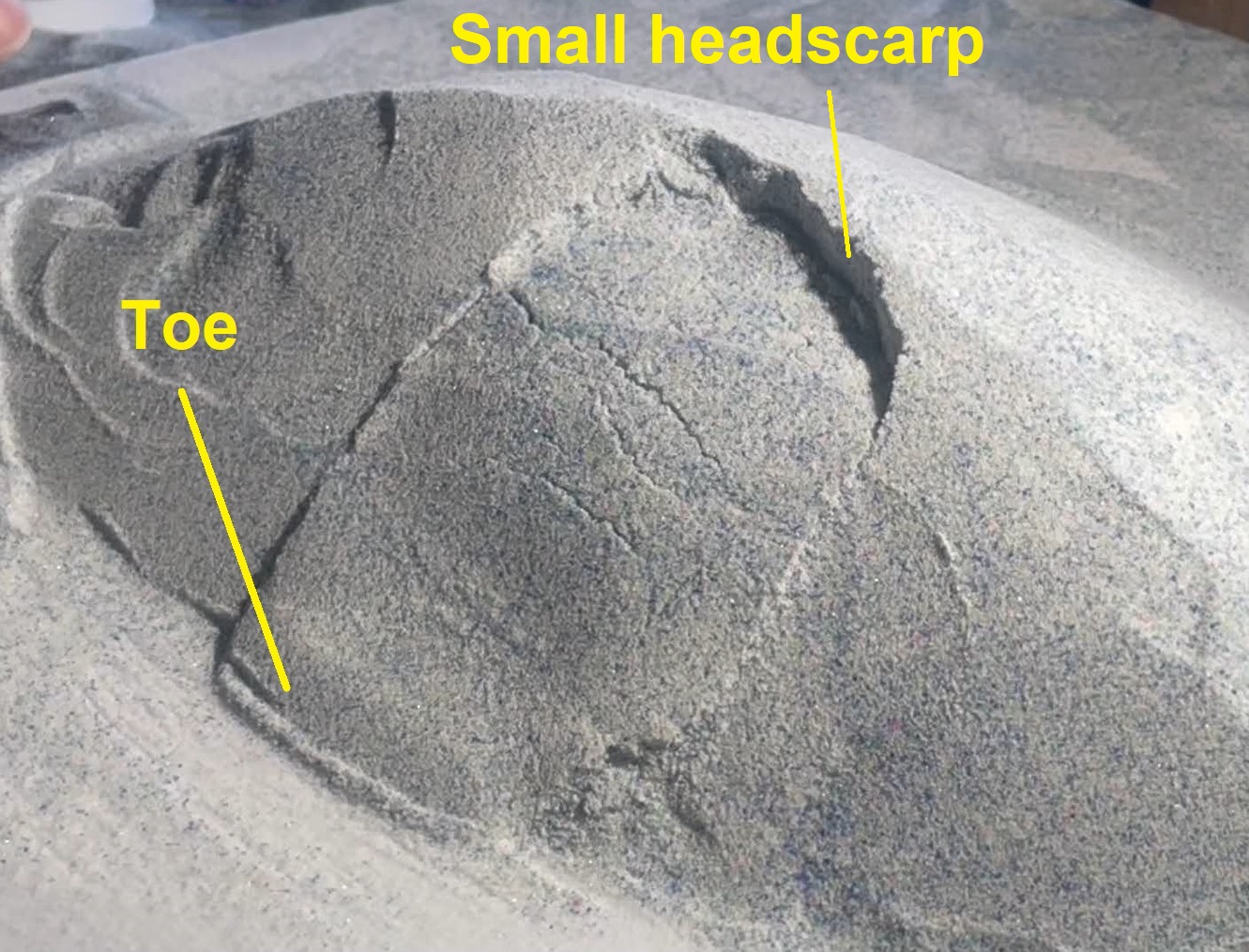
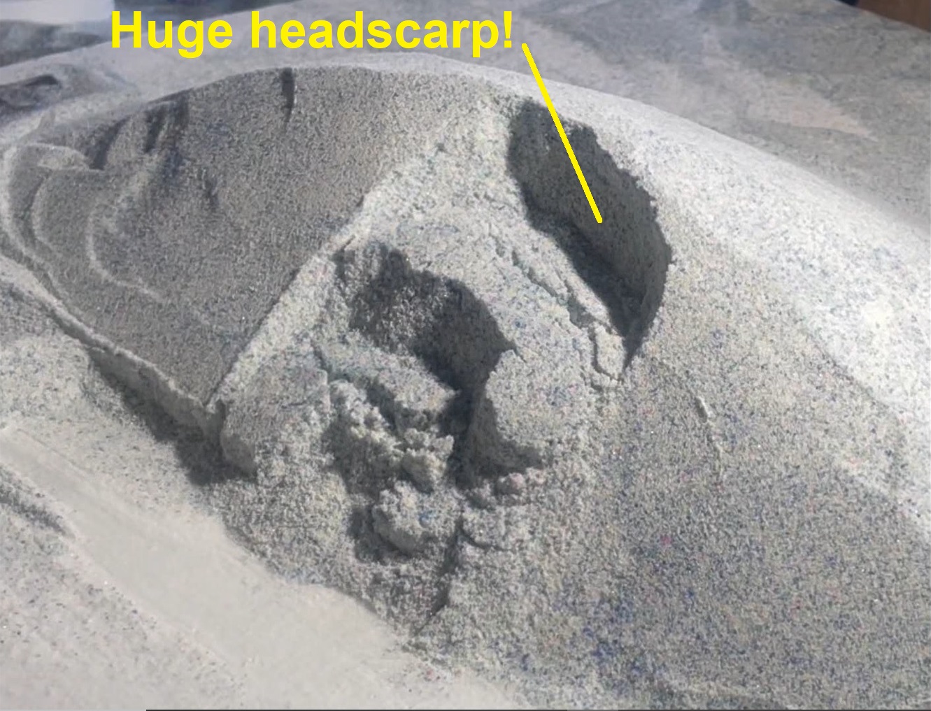
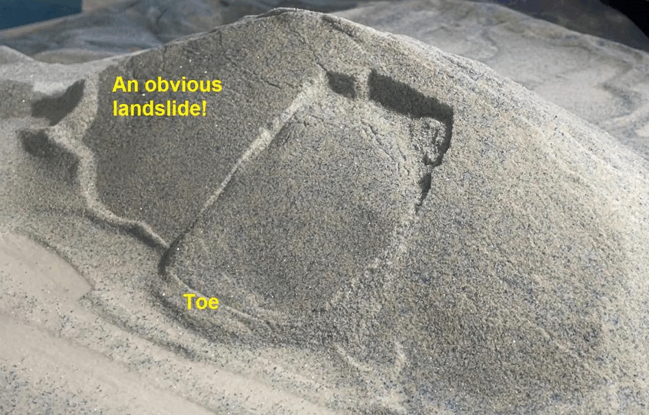
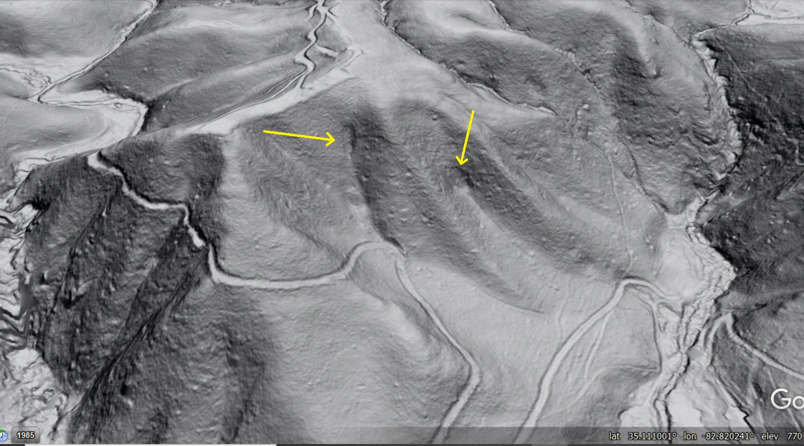
The slope above the Obey River shown below is a good example. The boulders looks small, but they are actually just shy of the size of the Pisgah boulder. Boulders this size are actually very common in this area, where soluble limestone beneath the sandstone caprock and a history of river incision set the stage for moving huge blocks downslope. The boulders shown below traveled as part of a larger landslide, but give the appearance of having moved independent of one another after the initial failure of the cliff line.
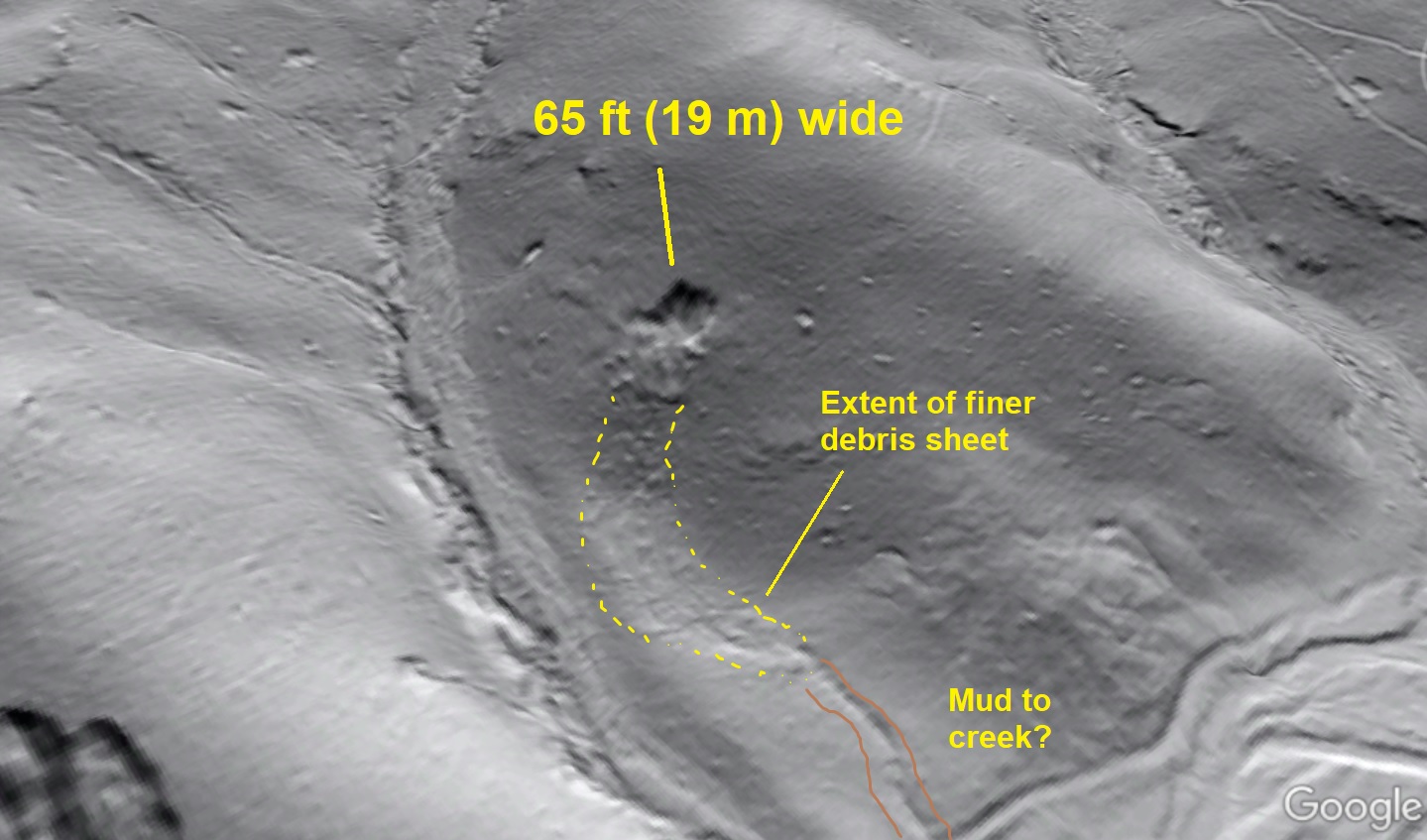
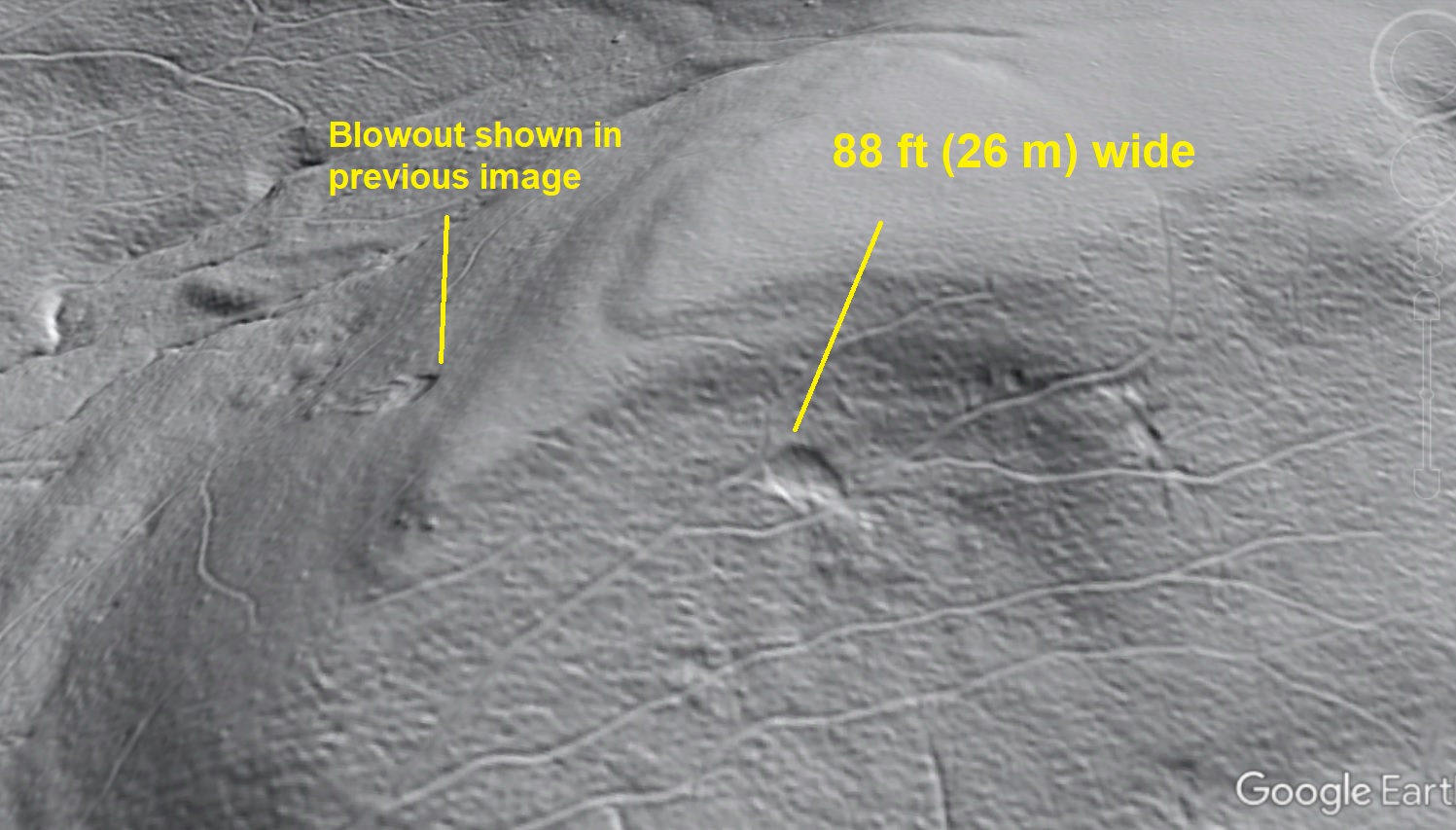
To the northeast, on the Big South Fork River near the Kentucky border, two large sandstone boulders detached from a cliff outcrop and plowed a clearly visible path downslope toward the river. the largest boulder, closest to the river, is about 115 feet long in its longest dimension.

A friend provide me with a photo of the 115 ft boulder, taken right at the end of the yellow leader line in the image above. Notably, these big sandstone boulders are not deeply buried in soil like the Pisgah boulder and Split Rock.

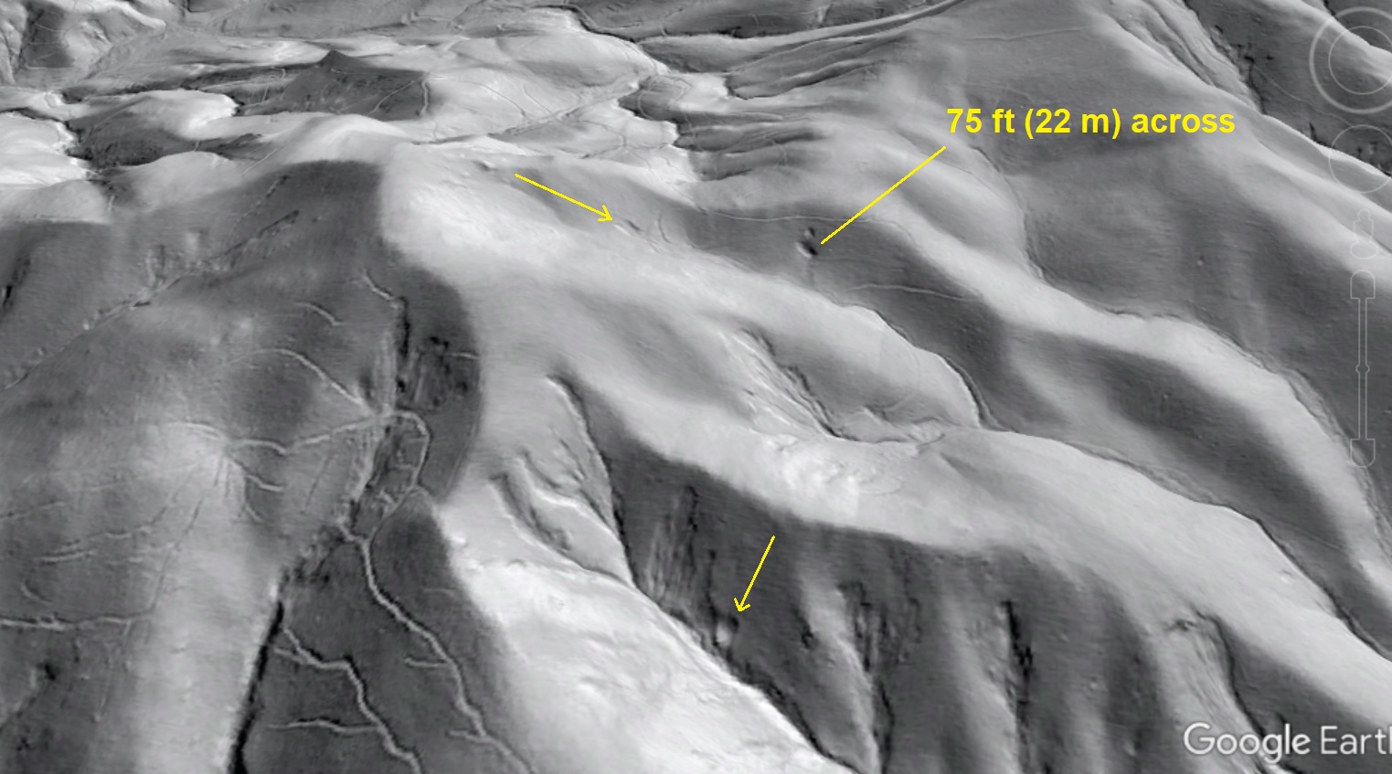
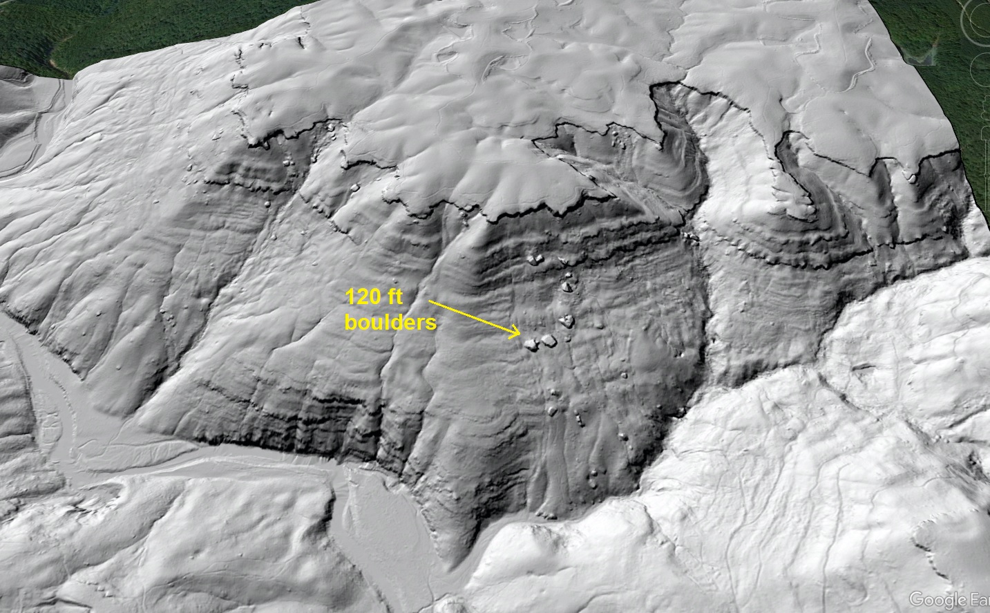
Further north in Kentucky, the Red River Gorge area is also full of ~120 foot sandstone boulders. The lidar shot below (taken from the Kentucky Geological Survey’s site) shows two 120-footers, indicated by red arrows. Boulders between 50 and 100 feet along their longest dimension are extremely common in this area. The joint-controlled, right-angle patterns in the cliff lines in this area are also interesting to check out.

The zoomed-in shot below shows the lower right boulder, which has traveled about 400 feet from the cliffline.

If you’ve paid attention to the measurements, 120 feet or so seems to be a common measurement for the biggest boulders to be seen in boulder-prone Appalachian landscapes. The Pisgah boulder and Split Rock aren’t alone in the southern Blue Ridge area; there are more 100-120 ft boulders to be found there, but they aren’t as numerous as boulders of that size in the Appalachian Plateau. In both areas, though, maximum size is intriguingly consistent, though only among boulders that have moved several boulder lengths from their source outcrops. Bigger chunks of rock can be found right along cliff lines, but these detached blocks have not actually moved or slid and experienced the associated physical forces. I imagine that the ~120 ft number is some reflection of the physical properties of the boulder-forming rock unit, both in terms of how it resists falling apart during sliding and how it controls topography to make cliffs and slopes to source and move big boulders. The image below compares sizes of the some of the boulders, with zoom adjusted so that it’s possible to directly compare them.

So, is the Pisgah boulder unique in any way? I think so. It is definitely at the top end of boulder size within Appalachia, though you can’t justifiably conclude it’s bigger than a reassembled Split Rock or something lurking in the Cumberland Plateau. It also traveled a significant distance from its source outcrop. This is notable because it contains aligned mica-rich layers that present plains of weakness along which it could break apart. The fact that the Pisgah boulder (and Split Rock) traveled hundreds of feet at their significant sizes and ended up in (mostly) one piece is impressive and probably the result of some amount of coincidence. Thick-bedded, very quartz-rich sandstone boulders lack aligned mica layers, so the potential to move a single huge piece of rock without breakup might be greater.
I don’t know how mechanical properties of the respective rock types would compare. Tensile strength of all Earth rocks is quite low compared to compressive strength, so rock doesn’t do well when forces try to pull it apart. Mica-rich zones or zones of extreme mineral weathering might lower tensile strength even more, so non-sandstone rocks might be less likely to hold together in single chunks than a physically hard and chemically tough quartz-rich sandstone. I also don’t know how these boulders move. I have always assumed that they slide, as tumbling would subject them to forces that would break them down to smaller pieces (that whole tensile strength thing, again). Check out what happens to the big block of rock in Switzerland shown below at this link.

Ultimately, geology superlatives (biggest, oldest, etc.) aren’t really worth much, but trends and patterns are useful in understanding how landscapes work. I looked at hundreds of big boulders, and not too much over 100 feet in the longest dimension is as big as you’ll see for a boulder that has moved significantly. This size is well-represented in certain sandstone-rich areas. Notably, sandstone-capped areas in Kentucky and Tennessee have, on average, bigger boulders than sandstone-capped portions of West Virginia. This may reflect local geologic details, climate and latitude, or both. The Blue Ridge serves up arguably the biggest boulders, though by an insignificant margin, and they are much less numerous due (presumably) to rock type details. Perhaps most interesting is that no one has ever seen a boulder the size of these biggies actually moving in the Appalachians, and none of them appear to be freshly emplaced. What makes them move and whether or not they do much moving under modern-day climate conditions is a big question in and of itself.