Note: This post is based on Jule Hubbard’s 2016 article, linked here. It’s a fascinating piece that does an excellent job capturing the human impacts of a notable landslide during the 1916 storm. You should give it a read before continuing…
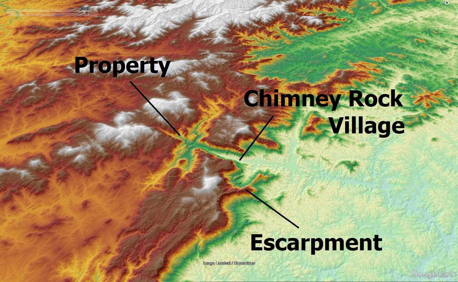
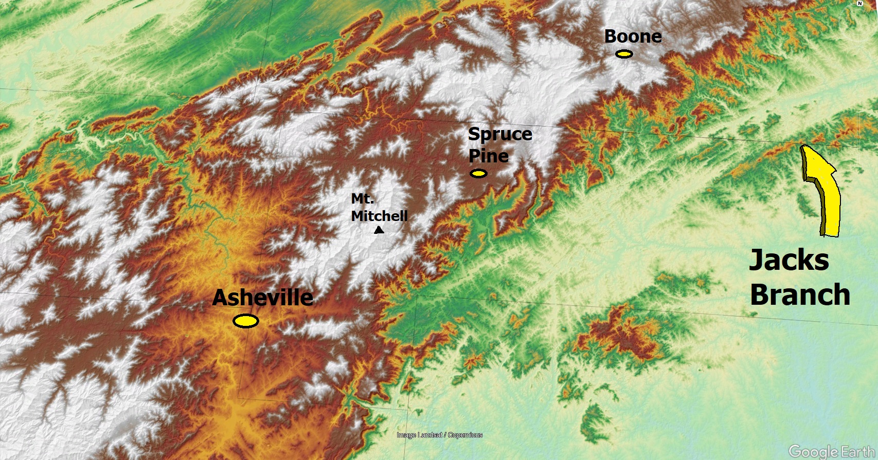
Prior to Helene, landslide geologists in western North Carolina devoted considerable energy towards studying the dual hurricane event of 1916 and the effects of such a “superstorm” on mountain slopes. Useful landslide information from the 1916 storm was–and still is–hard to come by, with stories maintained in relatively local oral traditions often providing the most detailed (and elusive) accounts. Jule Hubbard of the Wilkes Journal-Patriot skillfully developed written and oral records of one 1916 debris flow landslide into a 2016 article, linked at the top of the post. Interestingly, this debris flow occurred on a stream called Jacks Branch in the Brushy Mountains, a smaller range southeast of the Blue Ridge Escarpment and the higher peaks to its northwest.
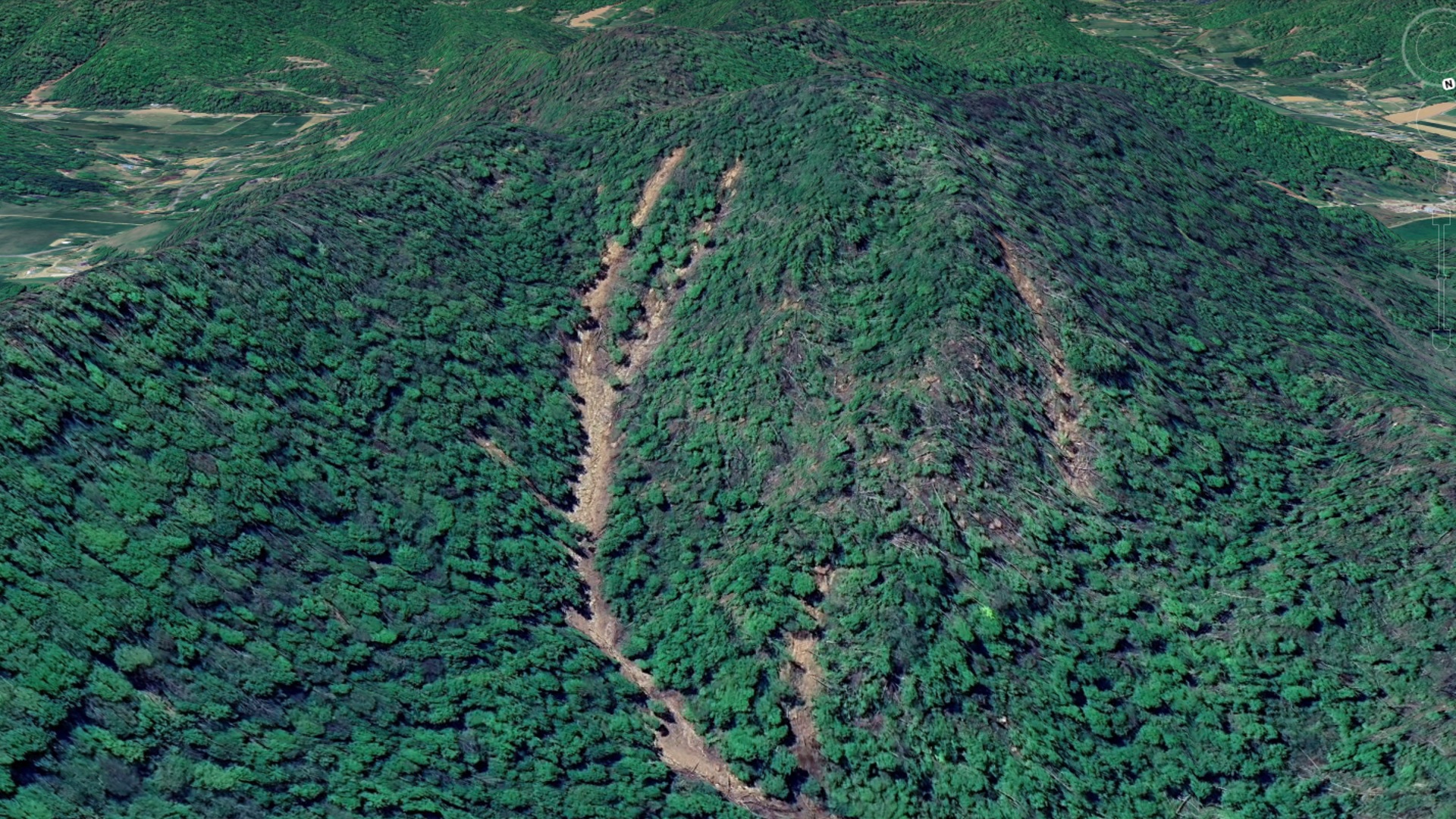
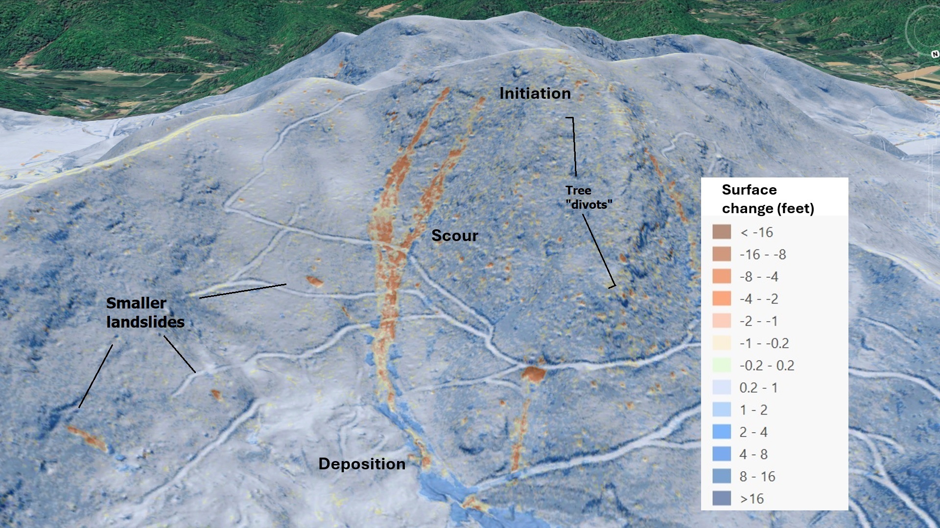
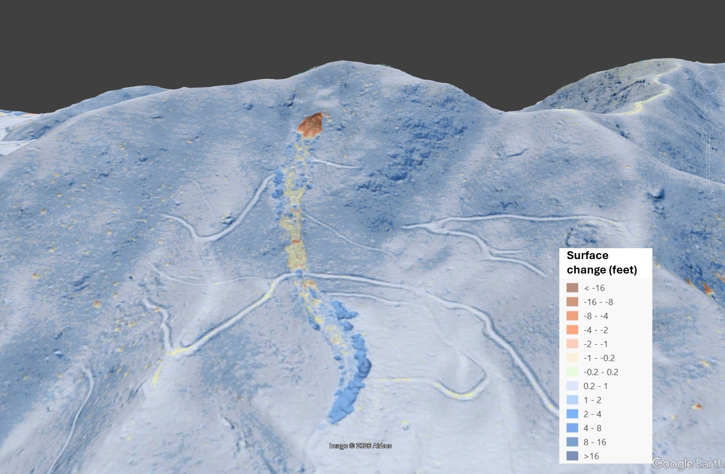
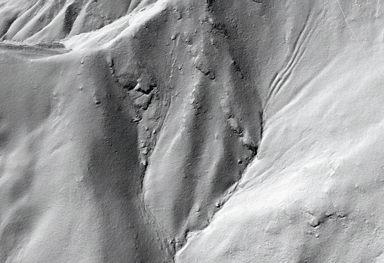
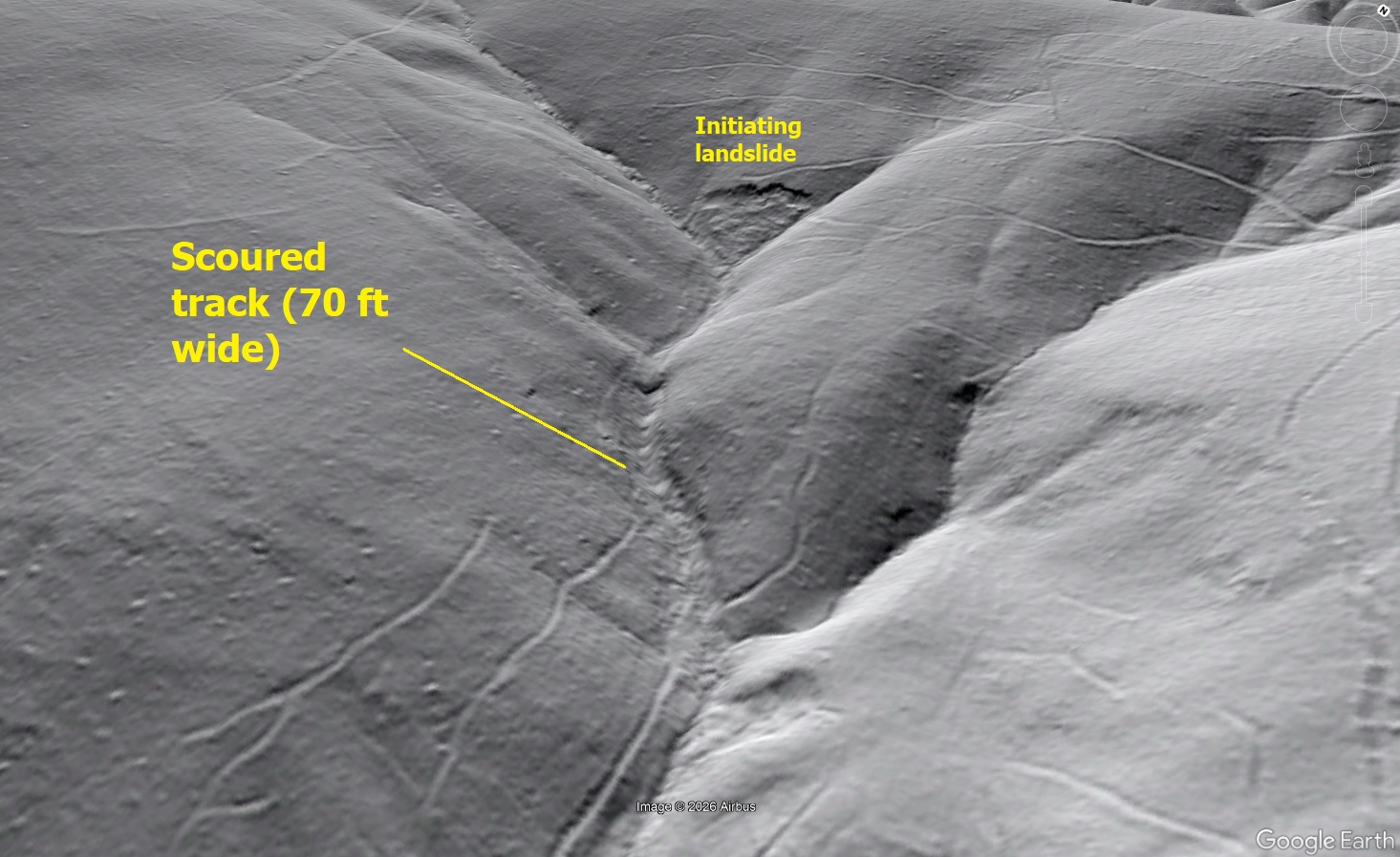
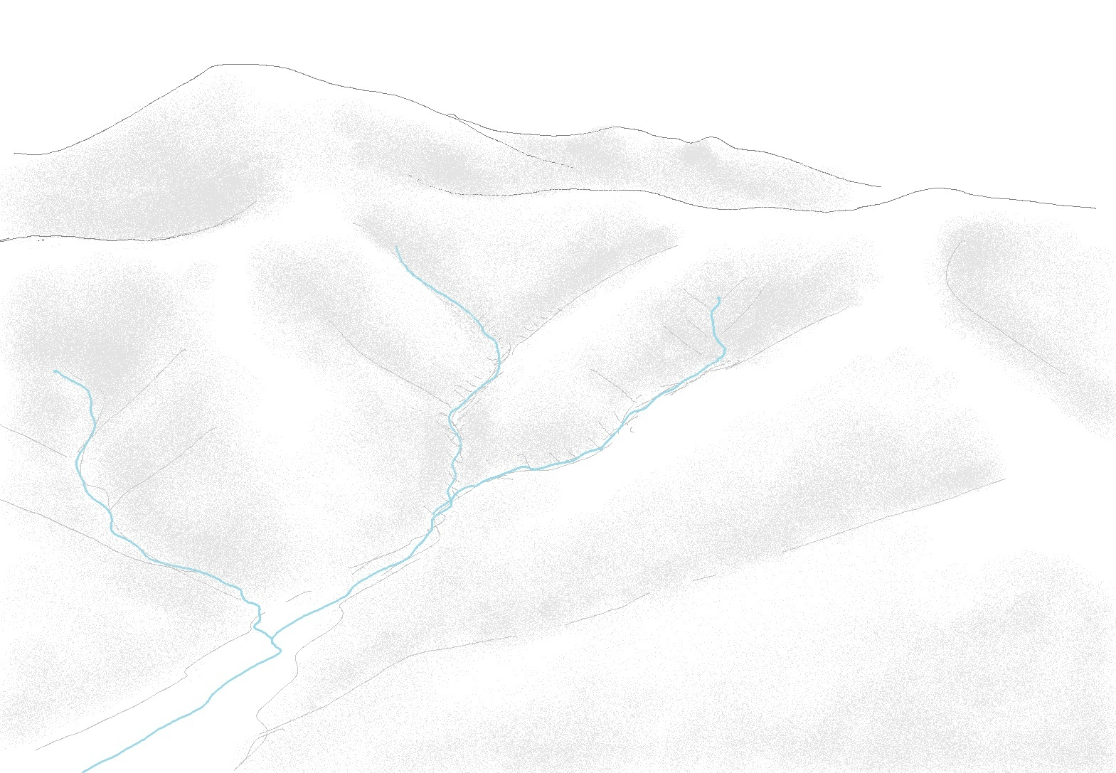
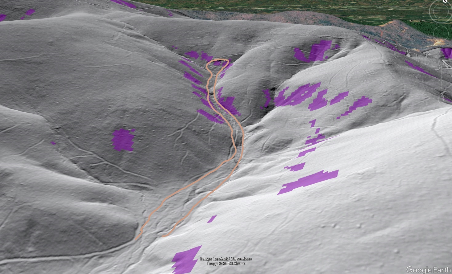
The Jacks Branch debris flow track remains clearly visible today, with significant scour occurring along a steep portion of Jacks Branch just below the initiating landslide.
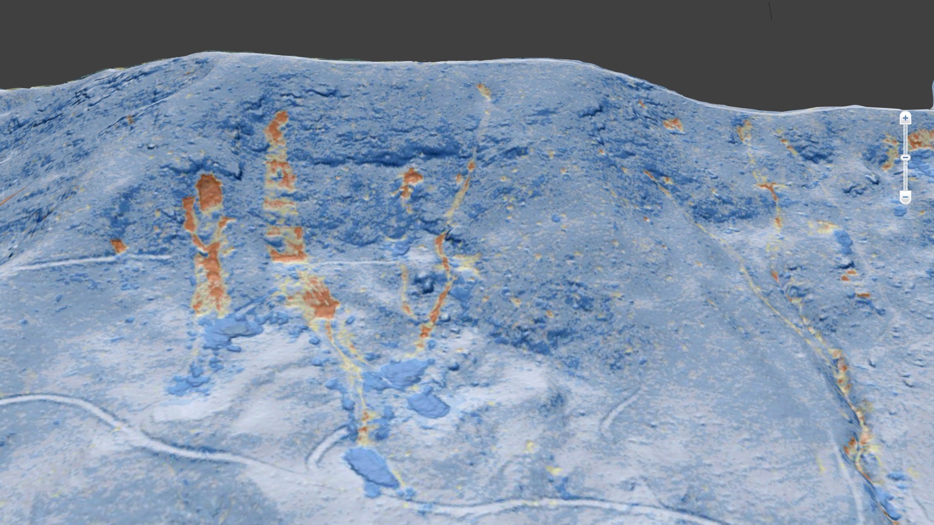
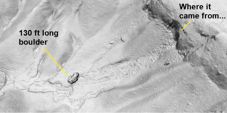
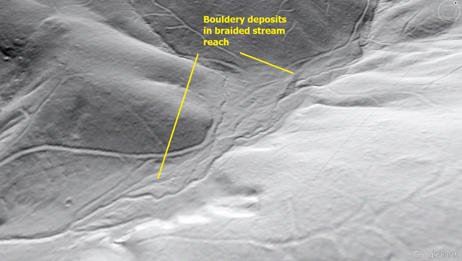
Below the scoured section, Jacks Branch has an almost braided appearance, with deposited boulders visible in 1-meter lidar imagery. The GIF below superimposes a 1/2 mile debris flow runout onto the lidar imagery, per description of the aftermath of the event recorded in 1916.
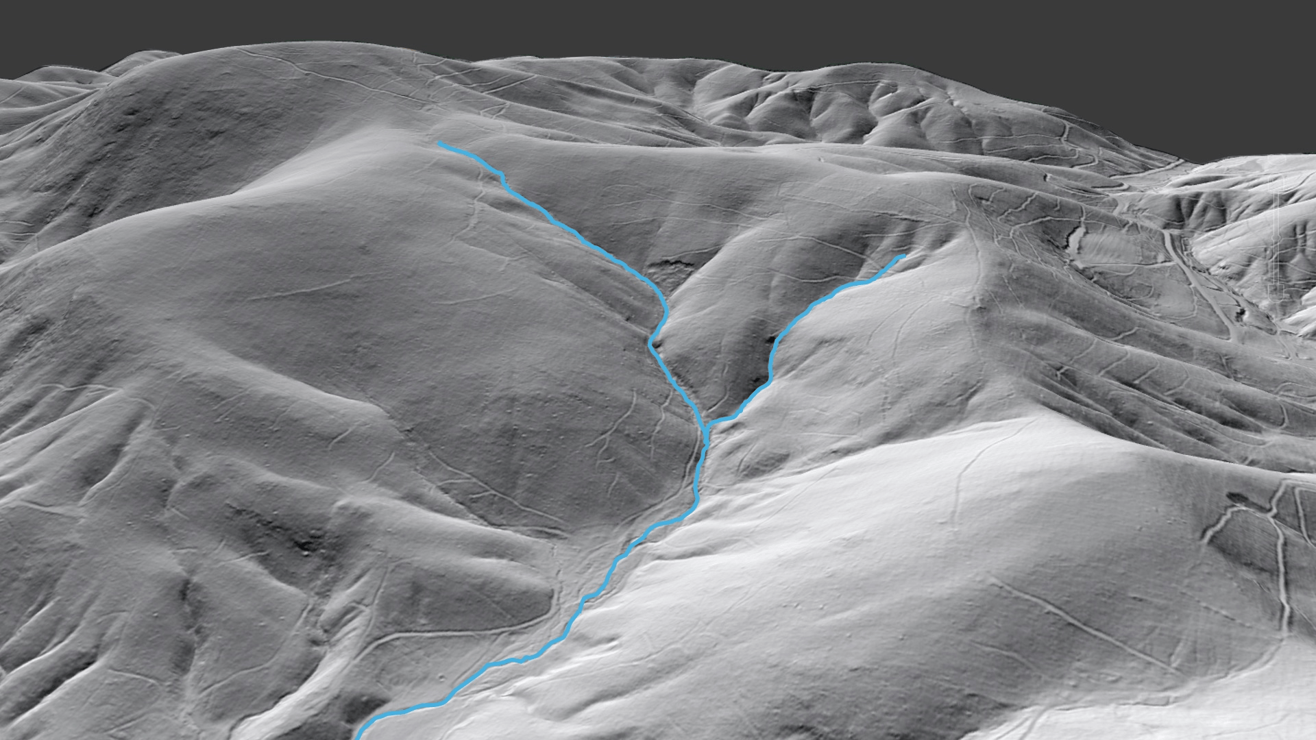
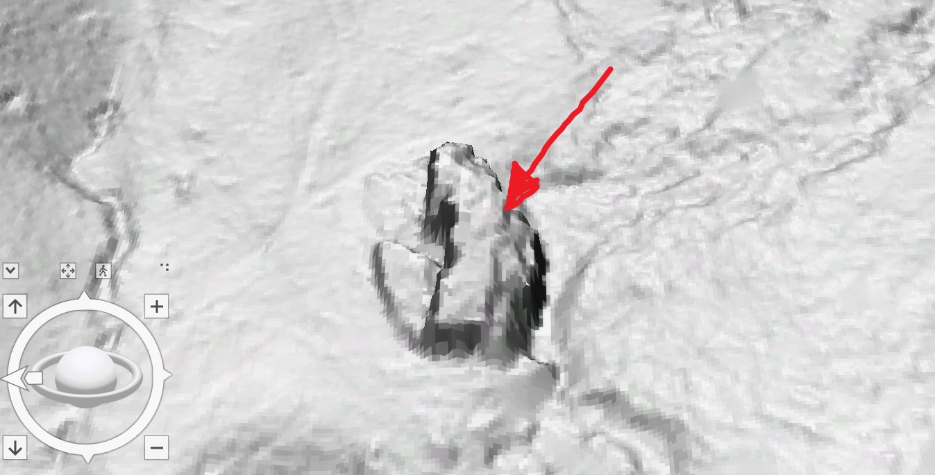
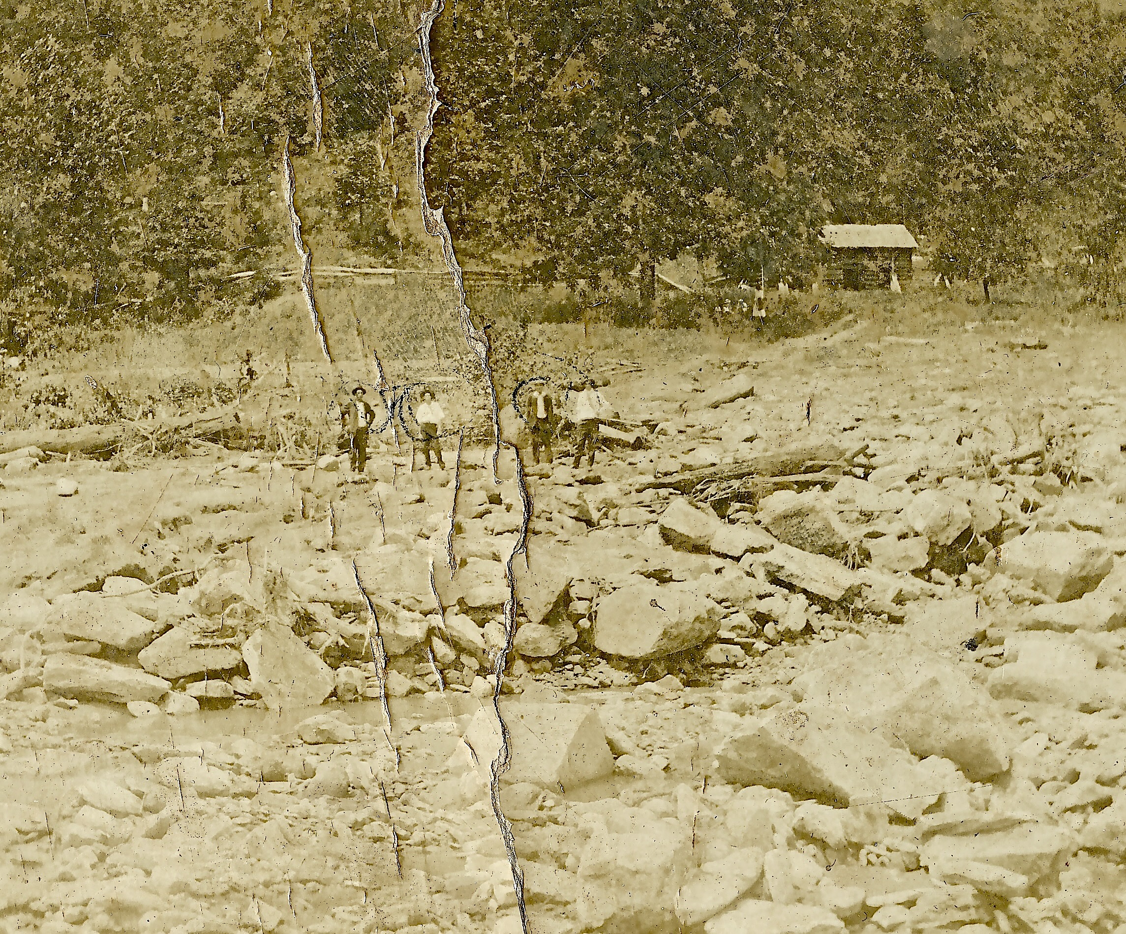
The 1/2 mile length appears to match the end of the braided channel and obvious boulder deposition fairly well, though a large amount of finer sediment likely continued downstream, mixed with floodwater. The lidar image below shows a detail of the bouldery ground surface, and the incredible 1916 photo, courtesy of Ann Loudermilk via Jule Hubbard, shows what the Jacks Branch aftermath looked like.
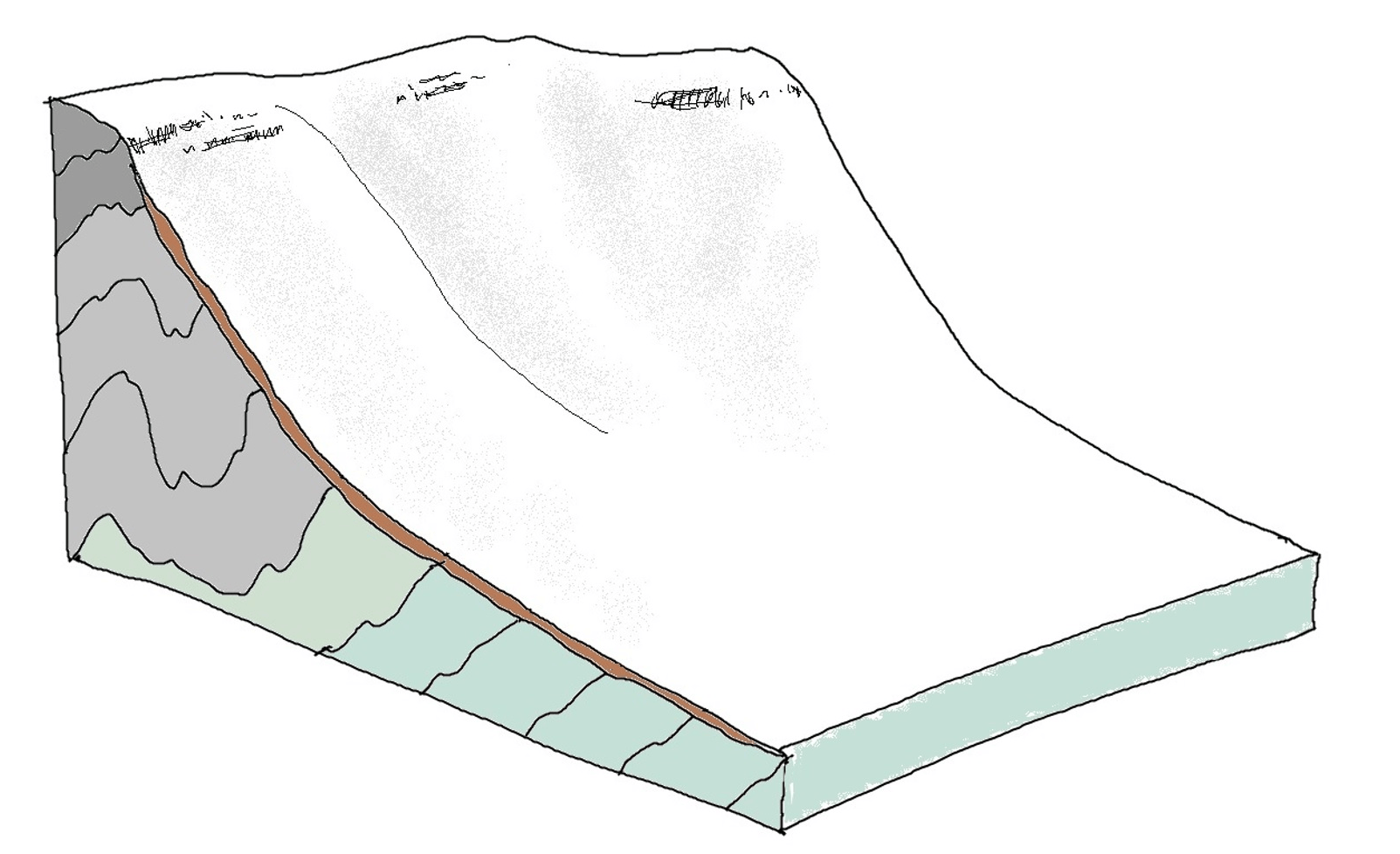
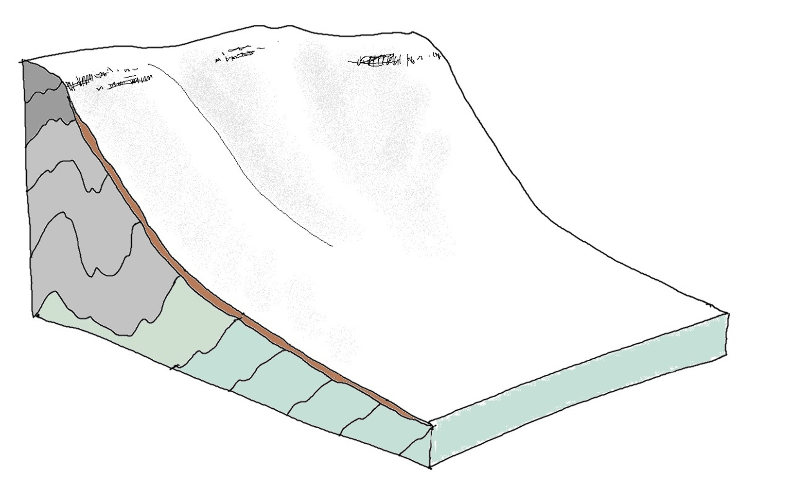
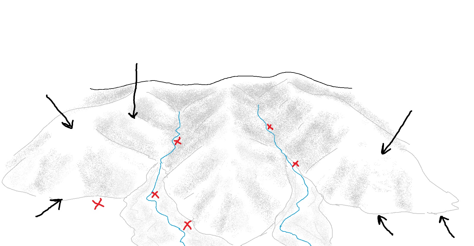
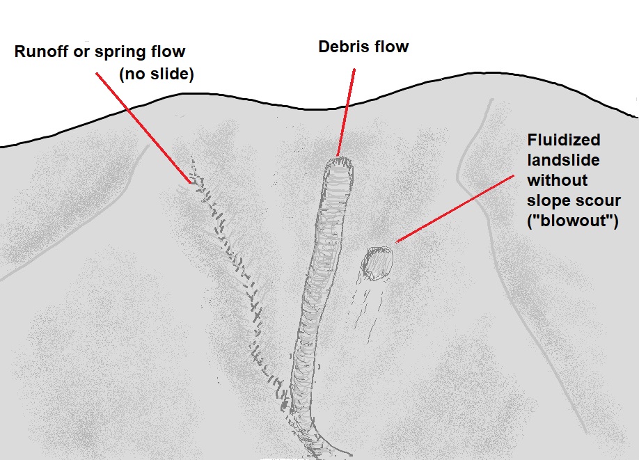
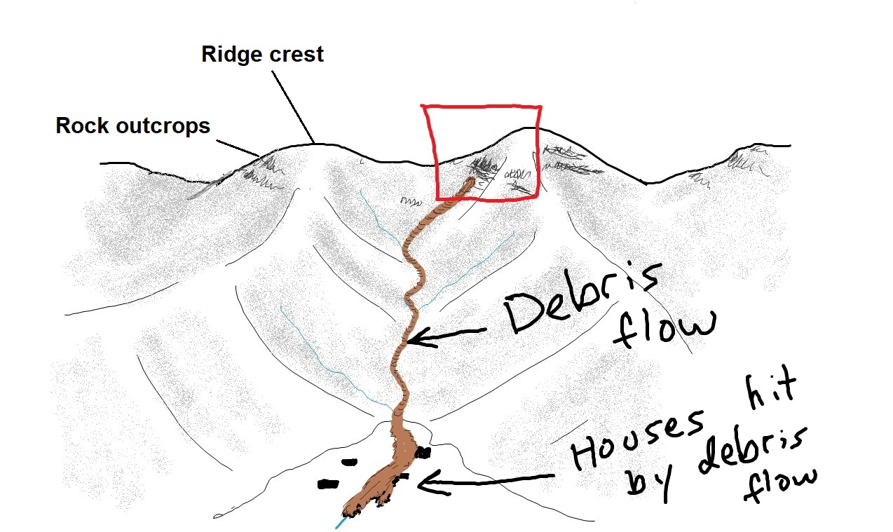
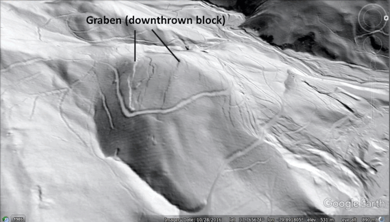
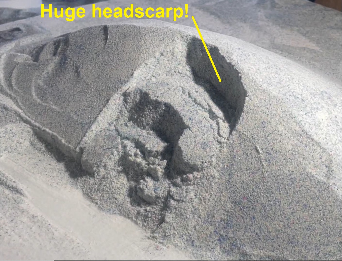
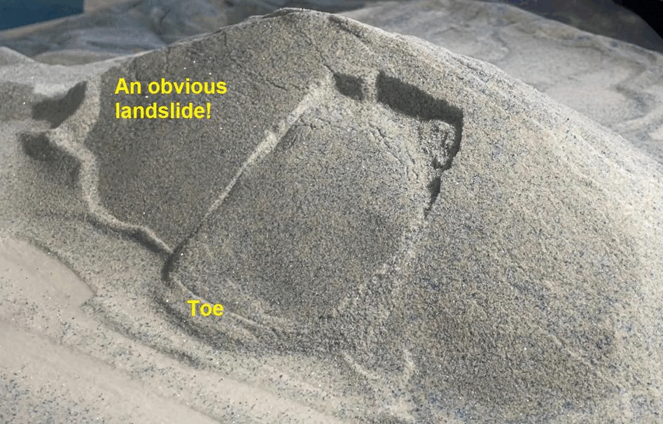
Locating this debris flow with lidar was initially a bit of a challenge due to the overall shape of the topography and atypical position of the initiating landslide. The scour of the Jacks Branch channel was the most useful identifier, whereas many debris flows of the higher Blue Ridge are first picked out by their initiating landslides within colluvial hollows. In the case of Jacks Branch, as with nearly all Appalachian debris flows, an initiating landslide triggers loading and liquefying of the saturated soil and rock debris along the channel downstream (more on this later). This “feedback” process produced an ever-growing mass of liquefied soil, rock, and trees, scouring the channel and delivering a huge amount of debris to the valley below. This GIF offers a conceptual animation of the process, along with the appearance of the aged and weathered track and deposit as it is seen in lidar imagery today.
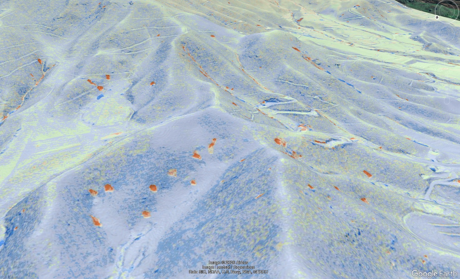
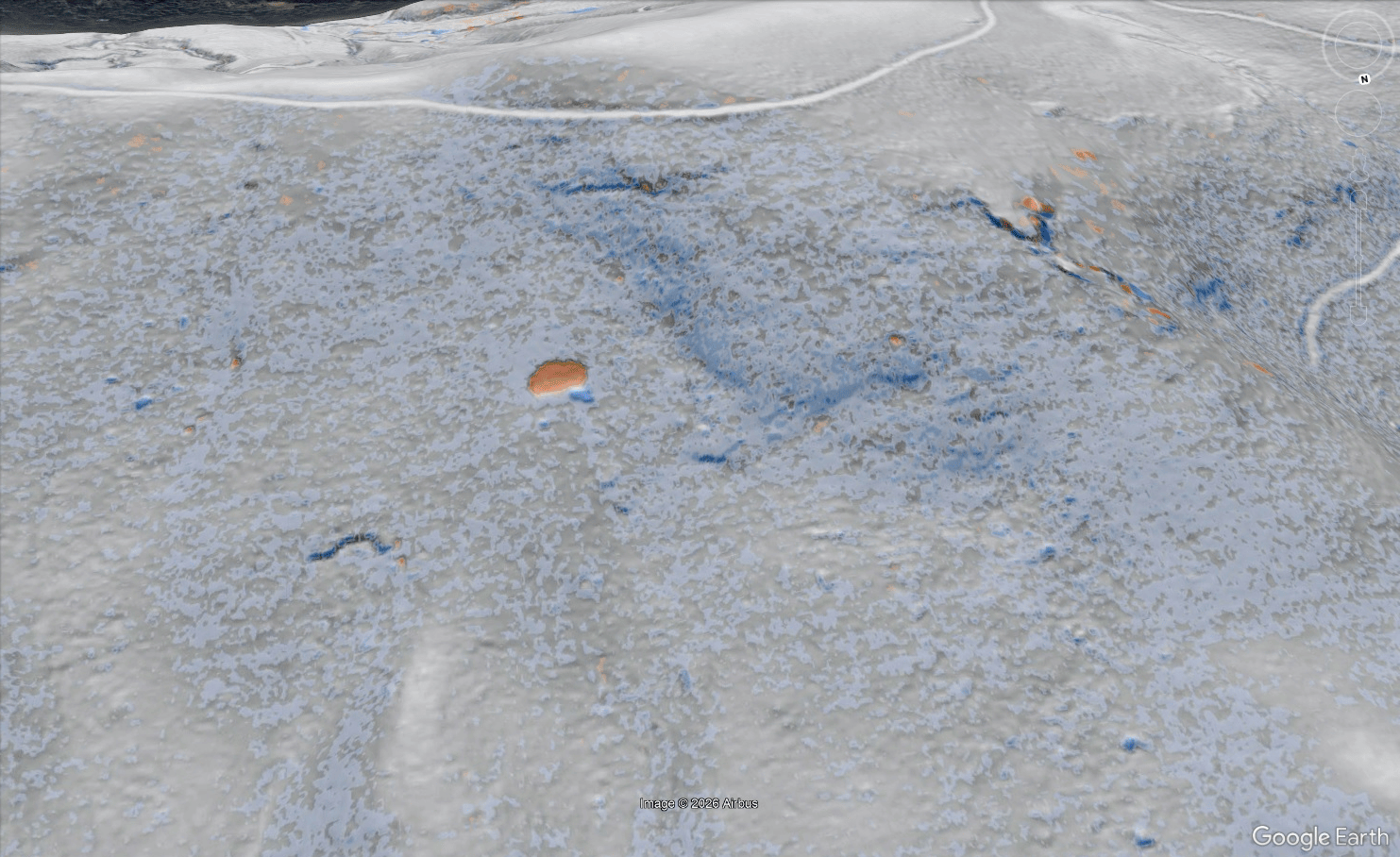
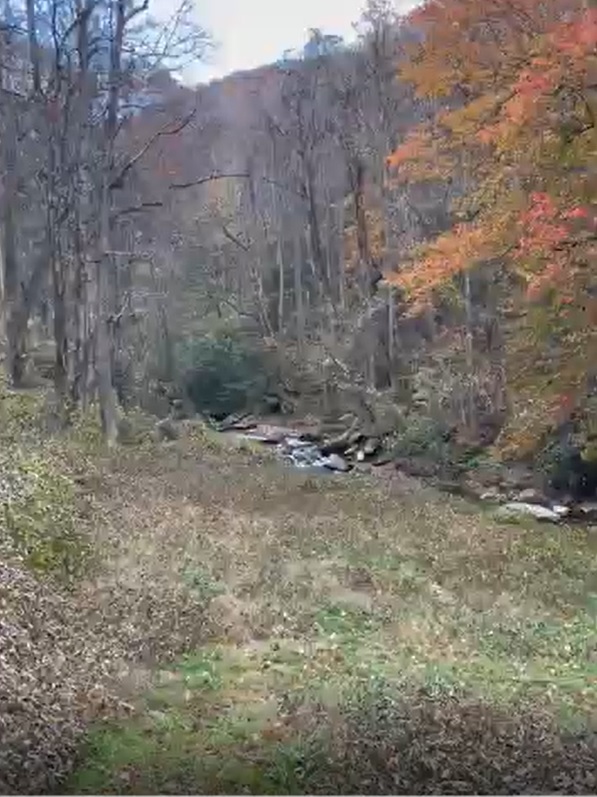
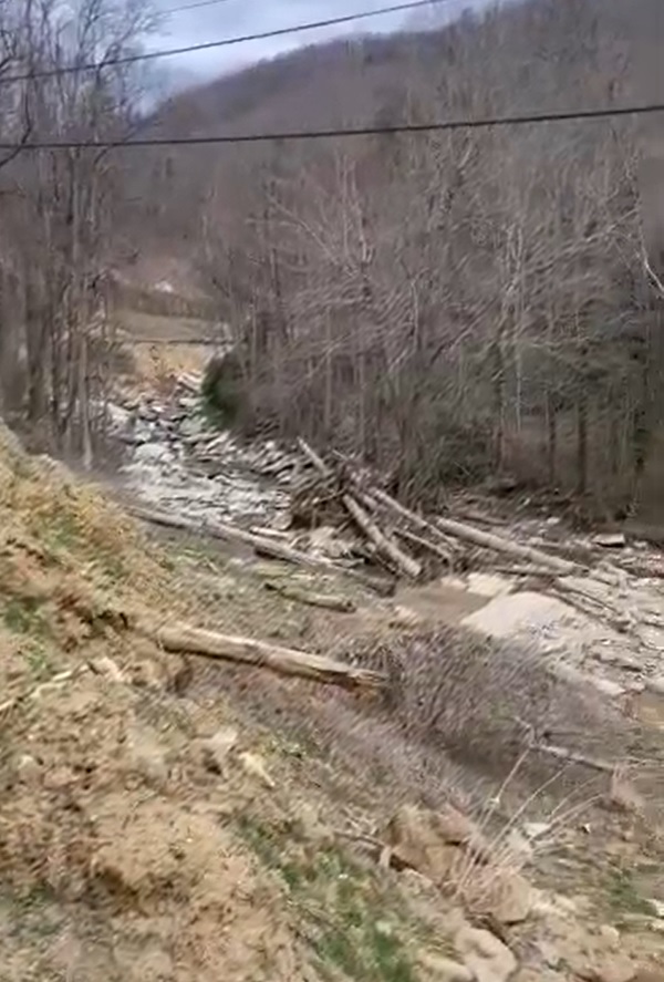
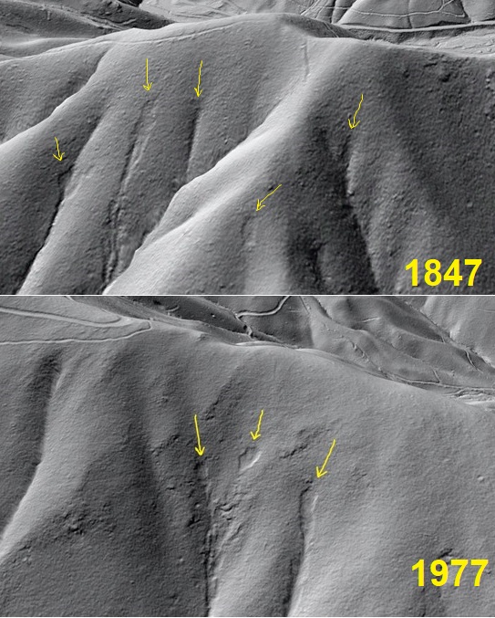
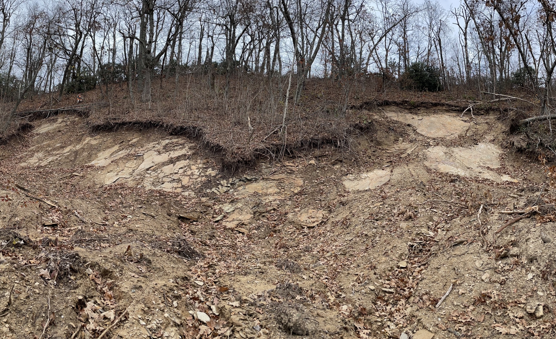
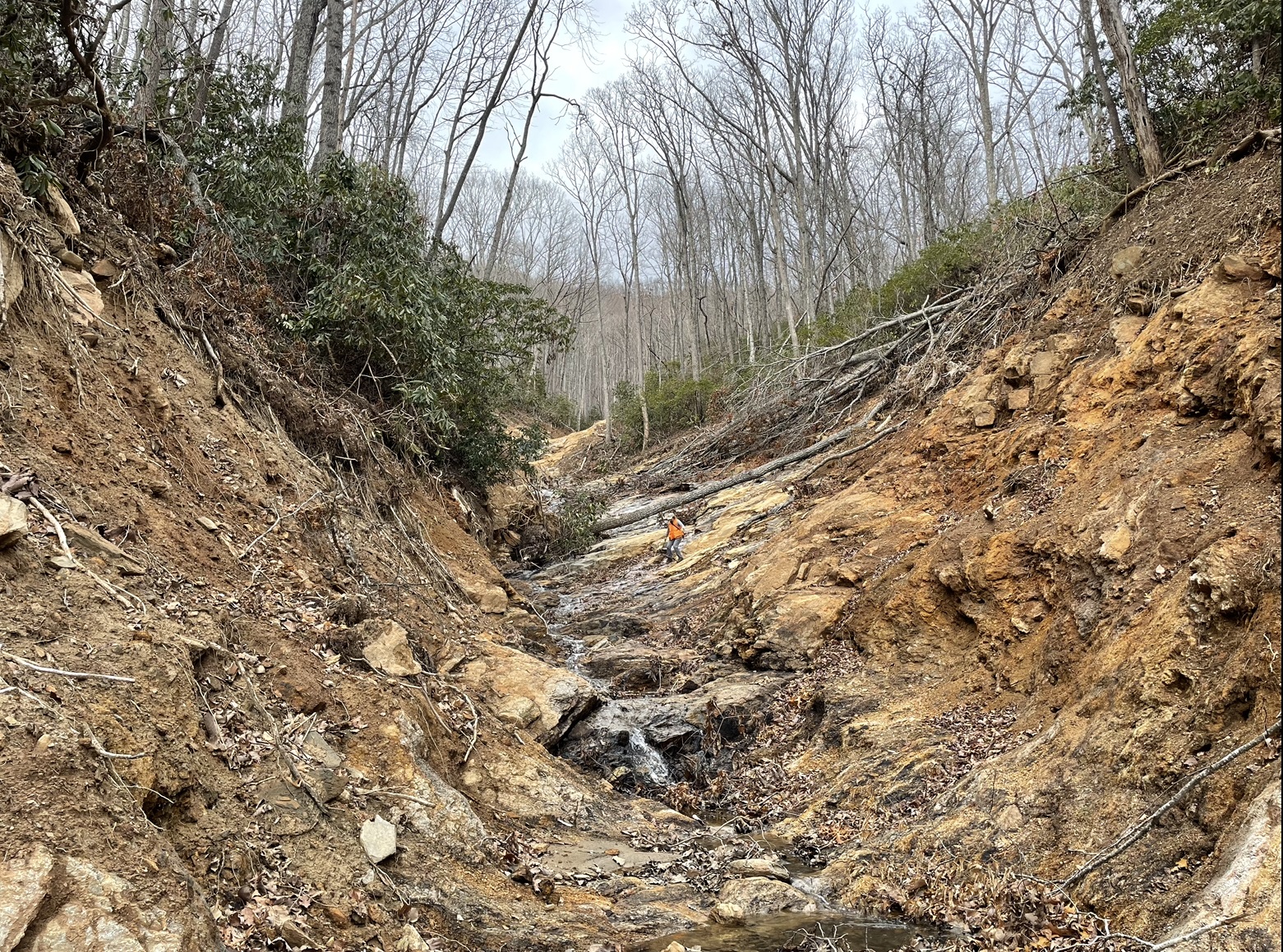
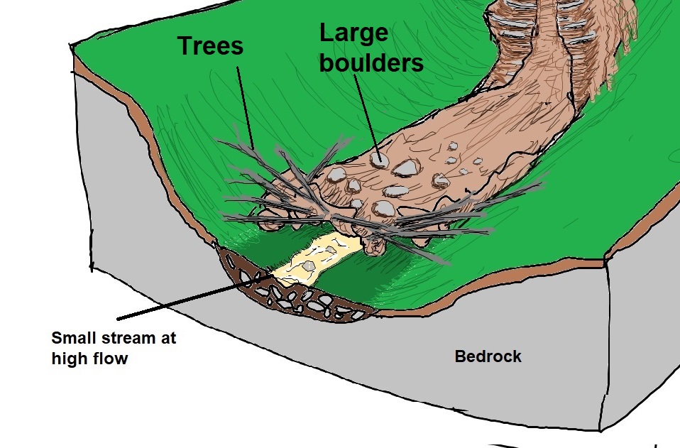
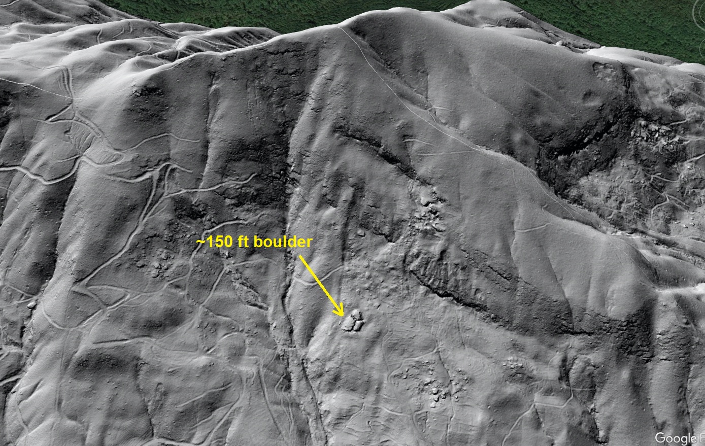
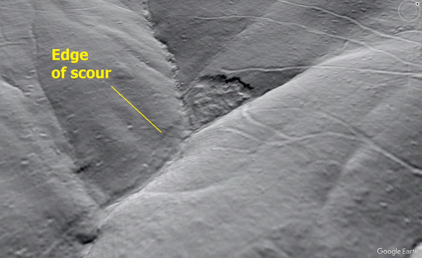
The scoured channel is quite impressive at 70 feet wide, even in the context of debris flows in the higher Blue Ridge that take advantage of longer, steeper slopes. The image below allows comparison of the scoured reach of Jacks Branch to an unaffected headwater stream. Prior to the debris flow, Jacks Branch likely presented a similar appearance.
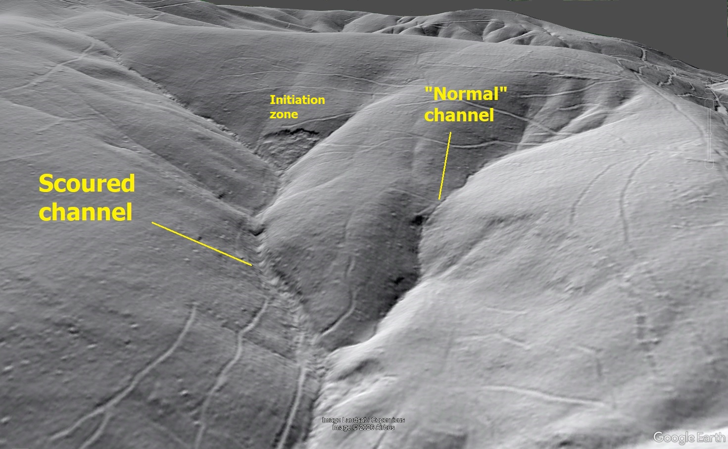
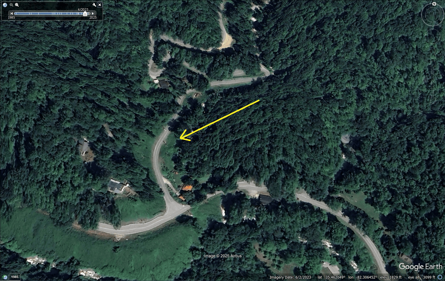
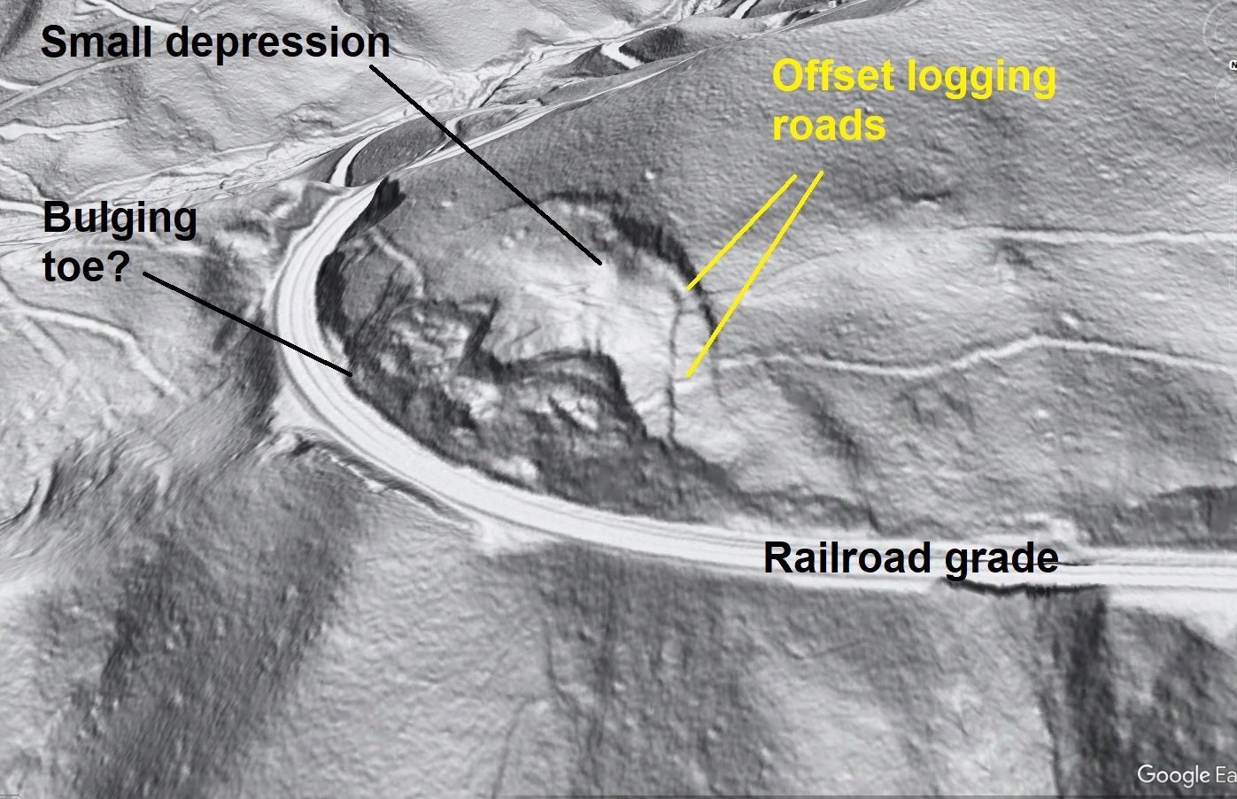
Scour can be seen cutting across the toe of the slope immediately below the initiating landslide.
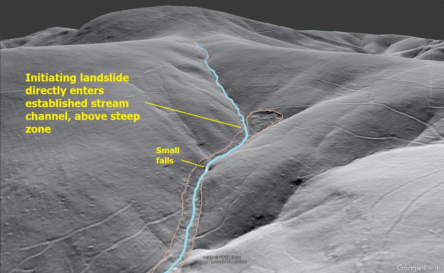
The Jacks Branch debris flow seems large in its scale and runout for the host topography, but we admittedly lack a large number of comparative examples to support such a statement. A notable aspect of the debris flow is that its initiating landslide entered the Jacks Branch channel well below its headwaters, causing the slide to enter an established stream that would have been moving a large amount of water at the time of the slide’s occurrence. Introducing the slide to the high stream flow may have aided liquefaction and mobility, or the slide may have briefly dammed the stream before its lower portions liquefied and initiated the debris flow. This second option may explain why much of the initiating slide is left behind (lumpy area in the image above), as the initiating slide of most debris flows in the region liquefies upon movement and leaves an empty scar. In either case, the flow promptly descended a very steep portion of Jacks Branch, where it gained mass and energy and headed for the valley below.
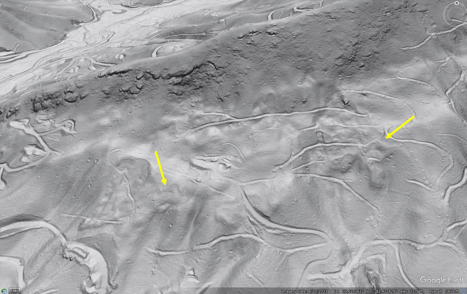
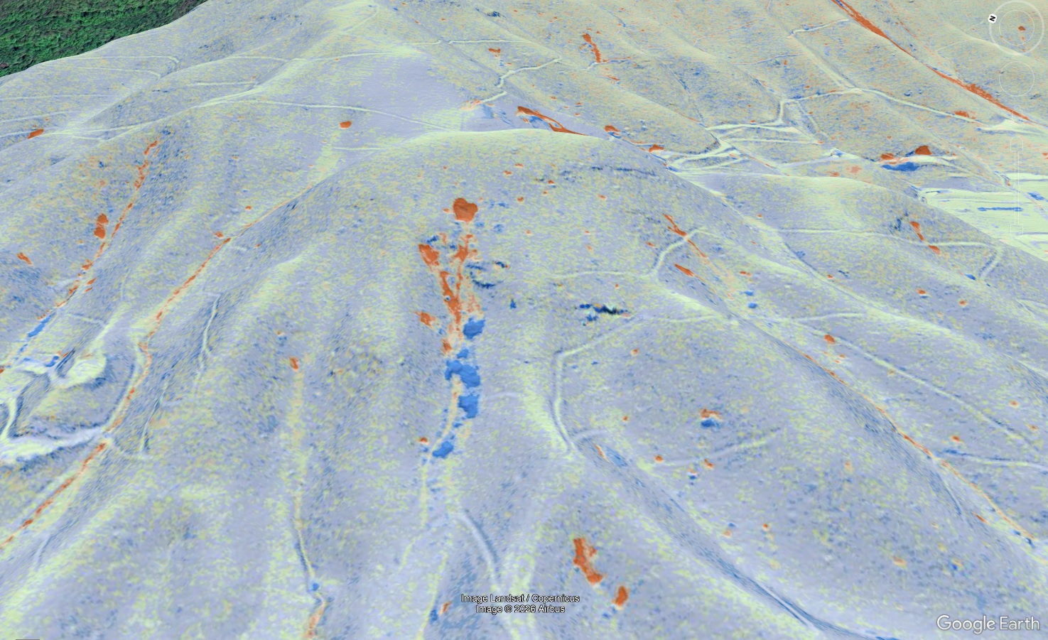
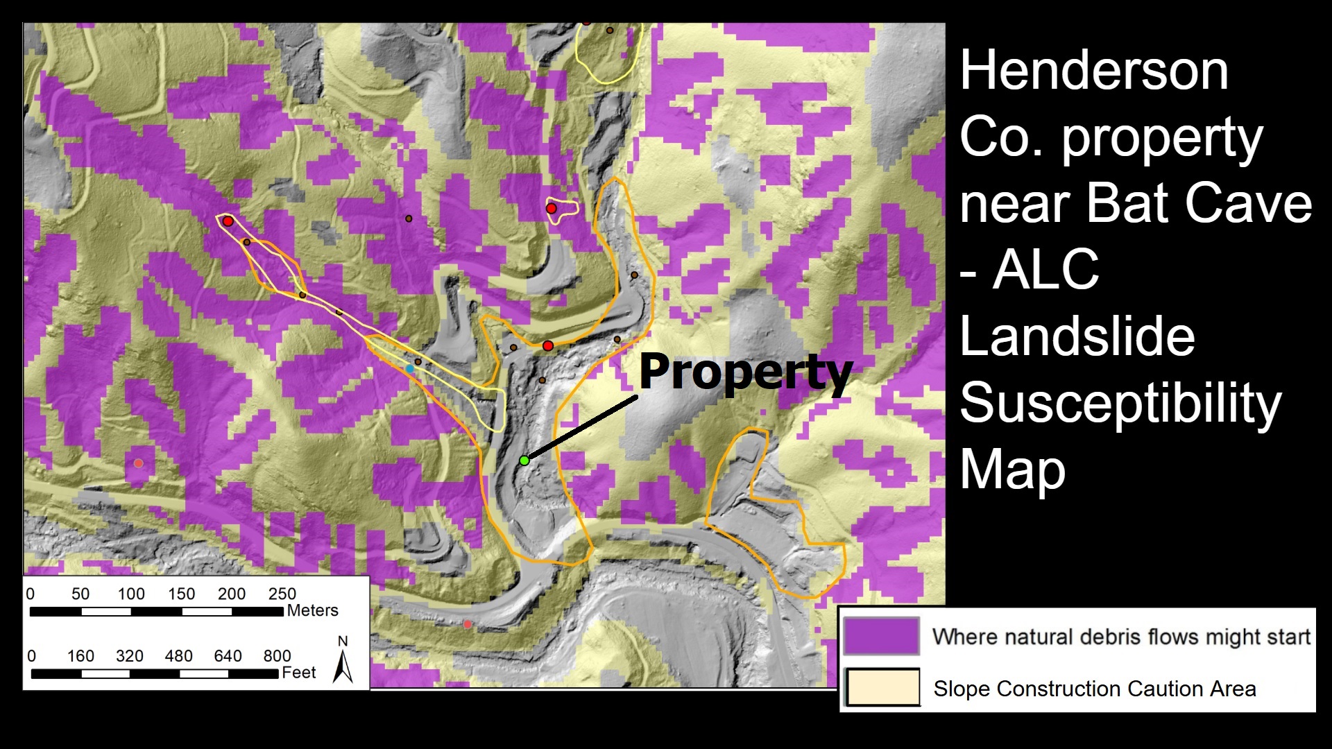
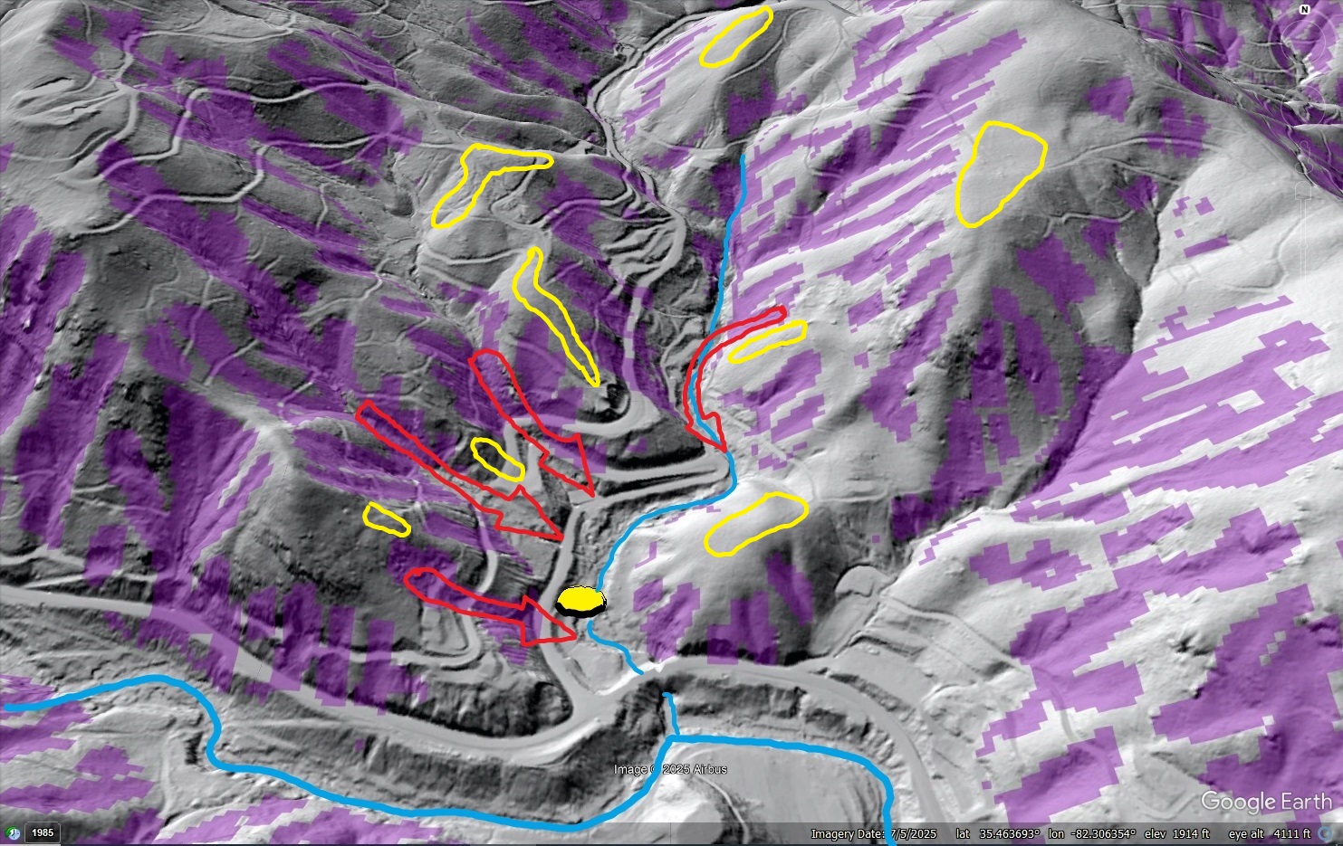
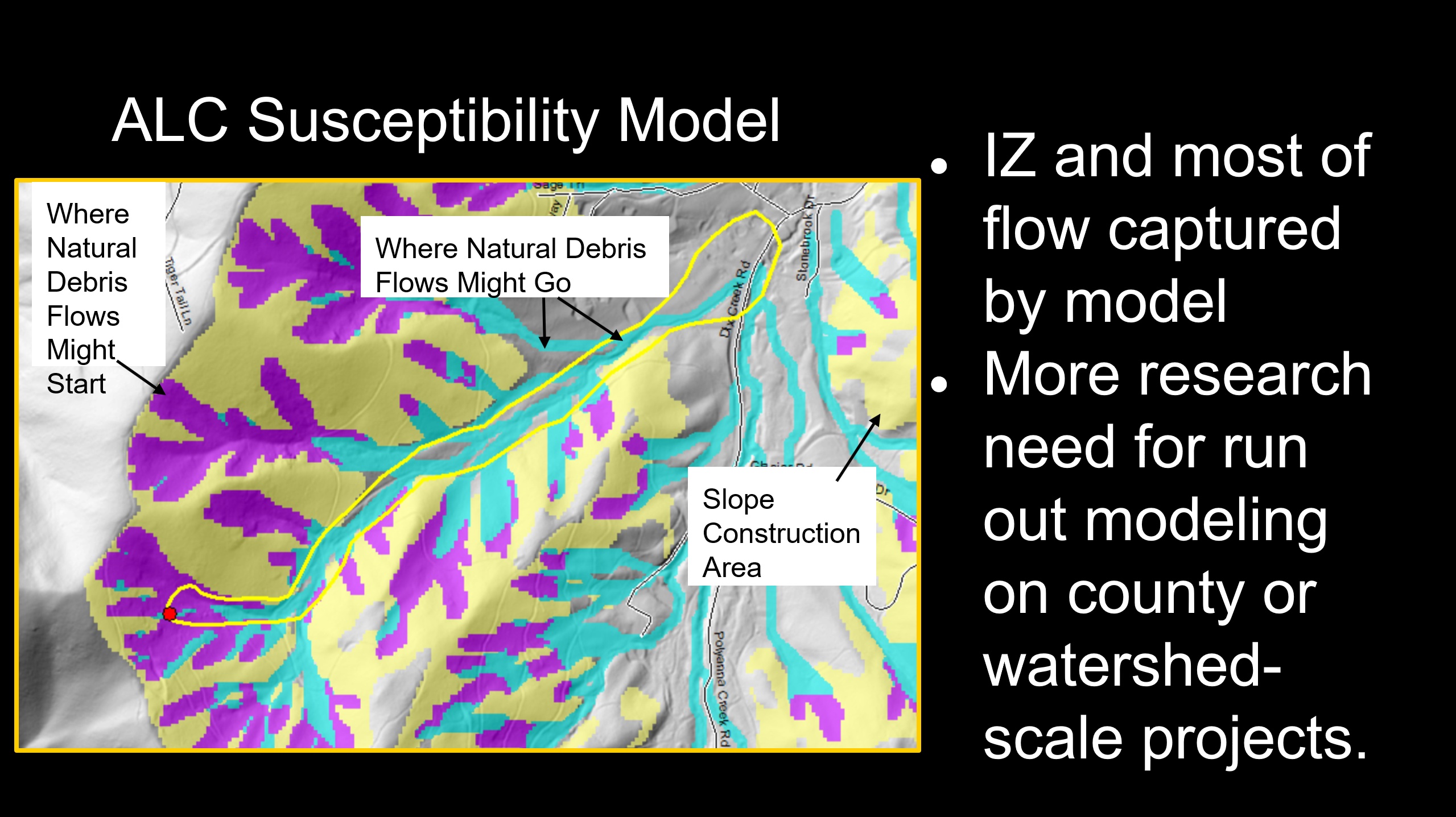
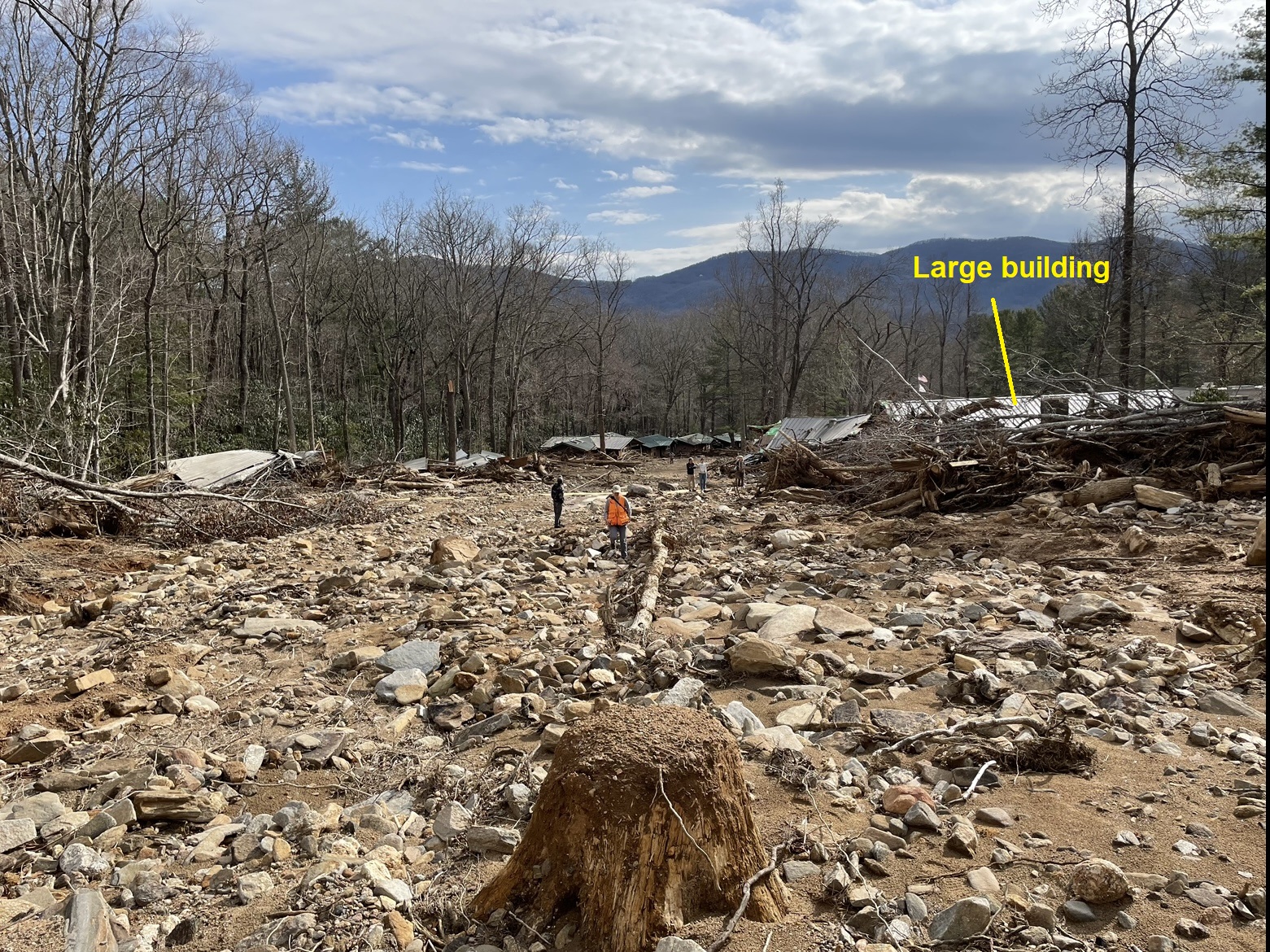
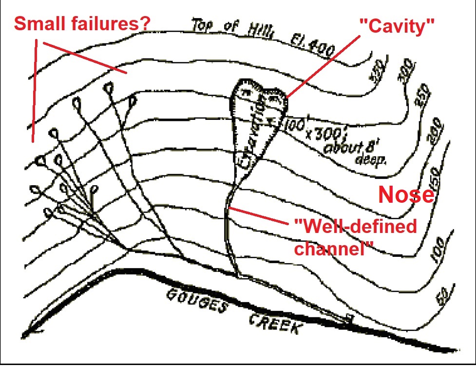
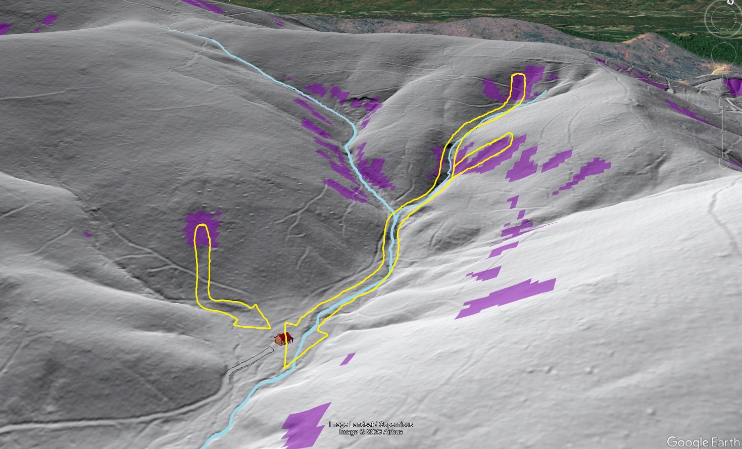
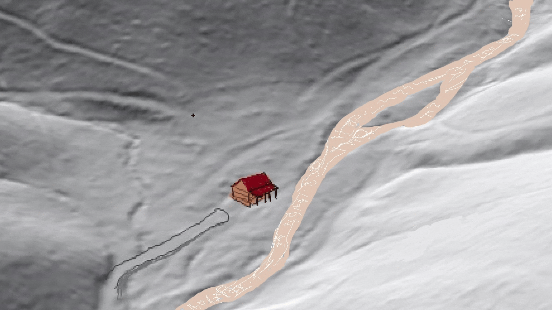
One detail that is lost to history (and can’t be answered from lidar imagery) is where the Russell cabin was located. One of Jule’s sources indicated that the cabin was located “on the mountain,” and not in the defined flat valley below. Somewhere near the confluence of the streams near bottom center of the image above is likely a reasonable location. The Russells obviously were not thinking about debris flows when they built or first occupied their cabin, and Jacks Branch or its tributary probably seemed too small to ever present a flood risk. I superimposed ALC’s Susceptibility onto the Jacks Branch area to see what we might say about building in this landscape today, given its distinctions from the high Blue Ridge. Areas where debris flows could potentially initiate (purple) do occur through the Jacks Branch basin, though in a somewhat different pattern from more rugged Blue Ridge landscapes. The Jacks Branch debris flow is outlined in brown.
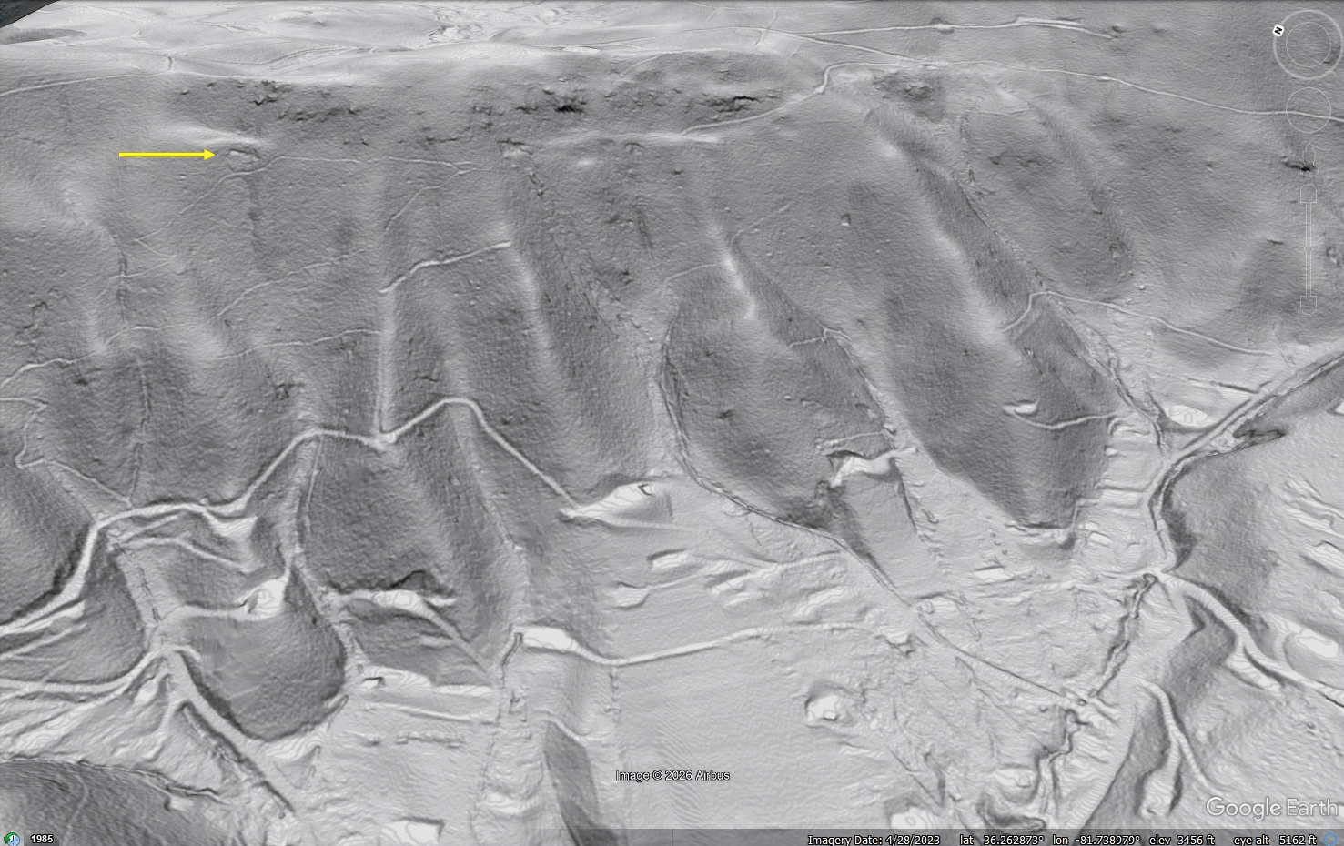
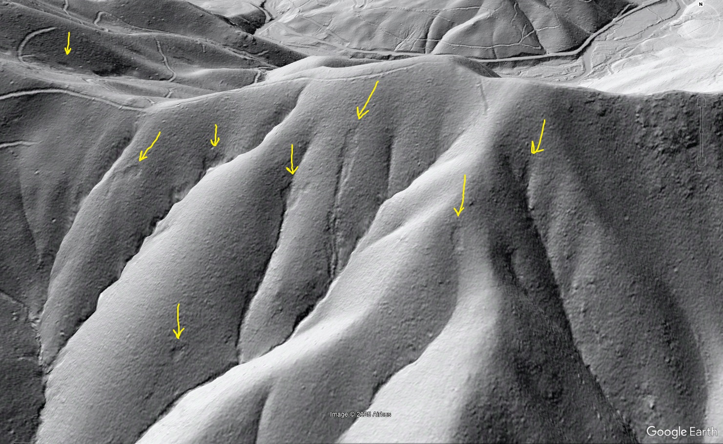
While this drainage basin is significantly less purple than many we look at, hazard areas are present, and debris flows initiating in them would follow the locally quite steep channels to the valley below. My pick for hazard the area shown above would be east (to the right of) Jacks Branch, in the steep, high hollows of the Jacks Branch tributary. A debris flow initiating there would ultimately end up in the same place as the 1916 debris flow, on the flat, deposit-filled valley below. While the flat valley area represents attractive, buildable topography that feels protected by the mountains, it’s quite vulnerable to debris flows during extreme weather conditions. The yellow arrows below show only a few of the possible debris flow pathways.
The Jacks Branch story is a valuable piece of history and an important lesson about steep slopes and extreme storms in the region. Huge mountains aren’t necessary for big landslide issues, particularly when rainfall and widespread soil saturation is sufficient to trigger debris flows. Debris flows tend to occupy MUCH larger widths than even the worst floods on the small streams they follow, leading to unbelievable aftermaths that suggest an impossibly huge “river of mud of rocks” suddenly appeared in a tiny valley. Linney’s account in the linked article communicates this idea very clearly. Avoiding the worst-case water flood on a small mountain stream isn’t enough if debris flow-prone topography is upstream.
Many similar stories undoubtedly exist in the region, and they all have their place in improving landslide awareness when the next “big one” hits, whether it is a tropical system or a one-off stationary thunderstorm. Anyone living in the mountains should take time to determine landslide hazard at their property and have a plan in place for when the “5 inches in 24 hours” threshold is likely to be exceeded.