by Philip S. Prince
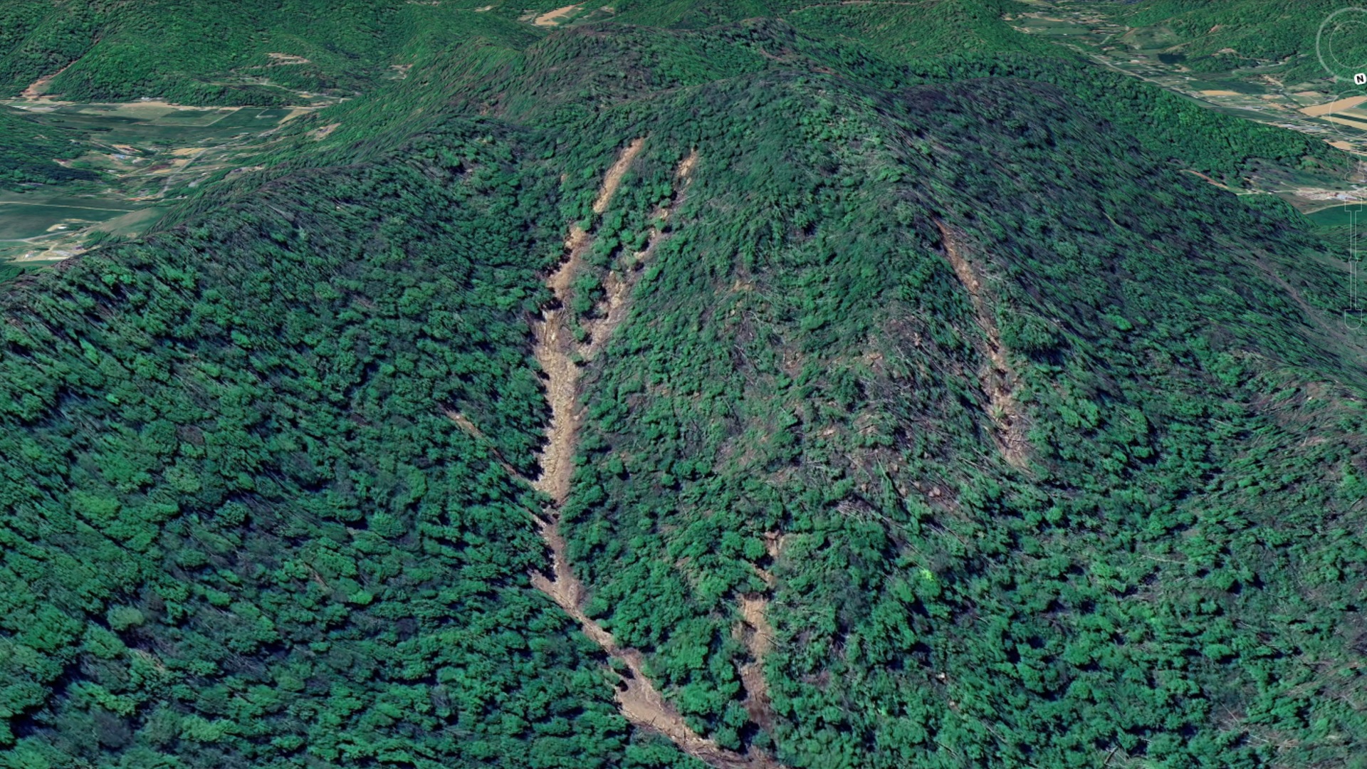
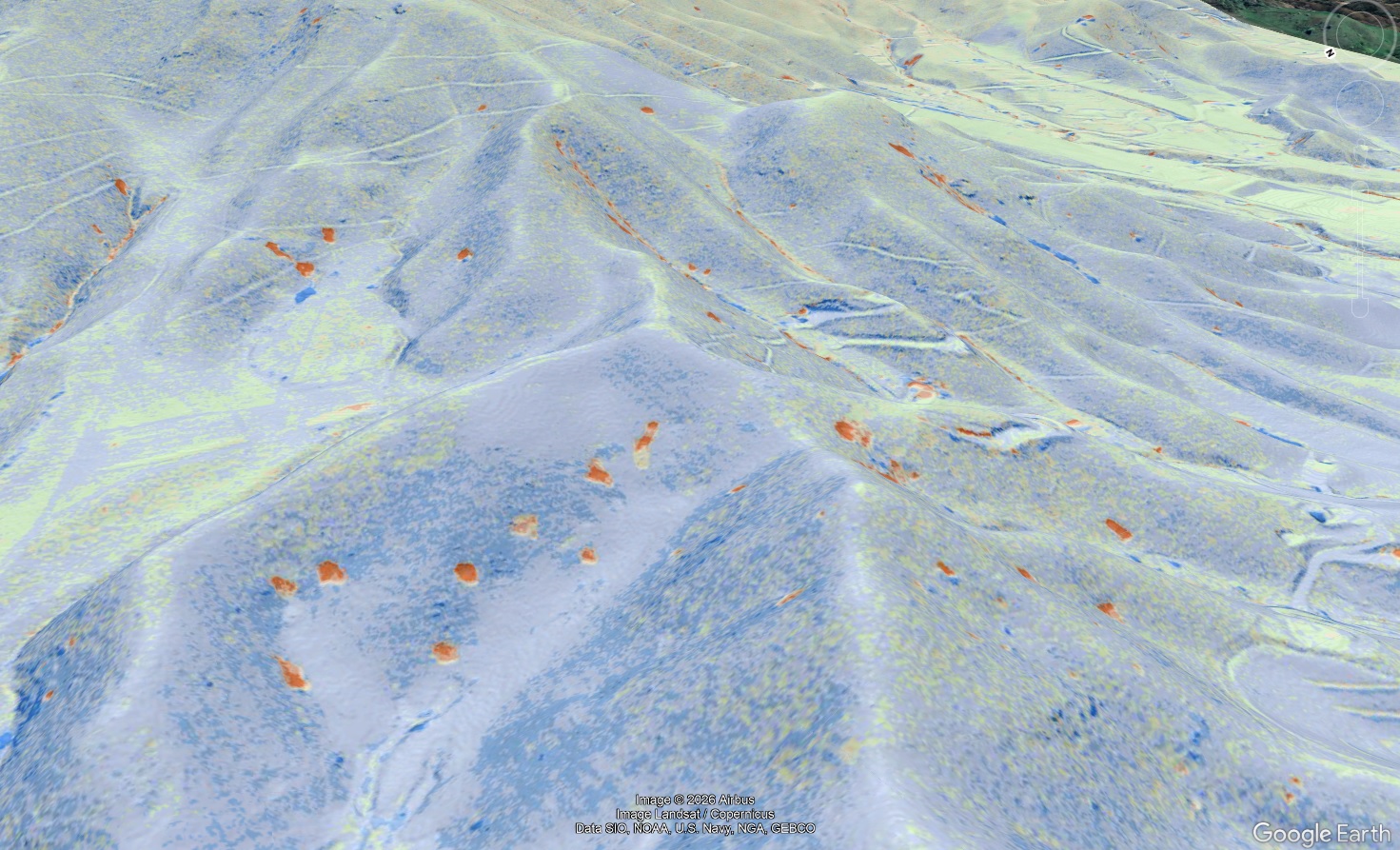
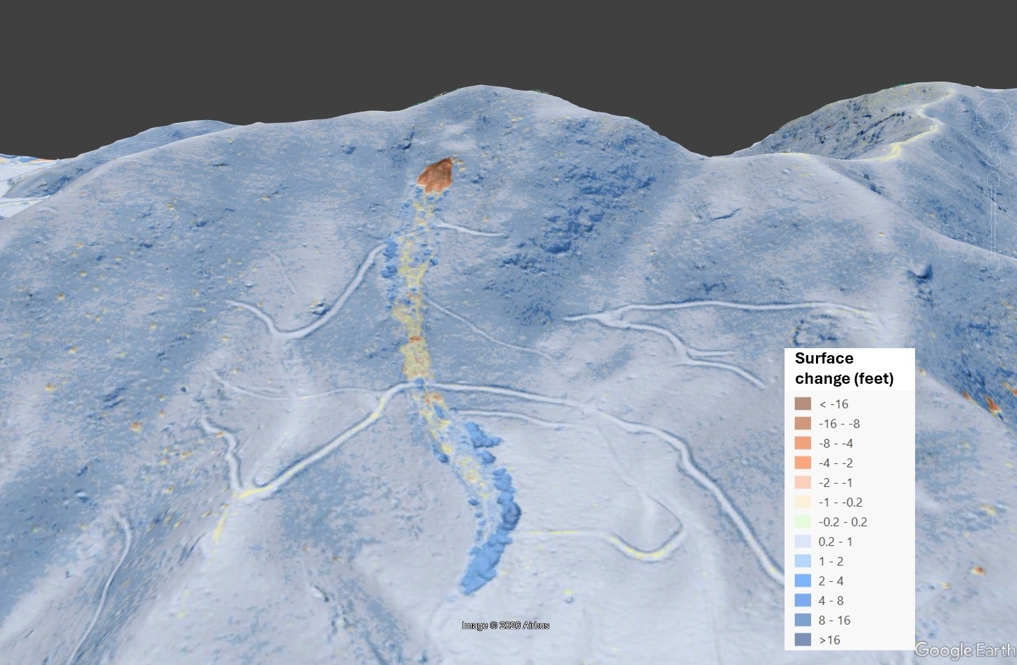
Over the last year, numerous collections of aerial imagery have shown Helene’s effects on western North Carolina mountainsides. This imagery has been useful in understanding the extent of the storm’s impacts on the landscape, but remaining tree cover and the natural irregularity of the landscape make it difficult to fully appreciate changes created by landsliding and flooding. Recently, long-awaited post-Helene lidar data has become available. Processing that data into imagery illustrating land surface by color coding loss and gain fully captures the storm’s effects. ALC Principal geologist Stephen Fuemmeler has produced county-wide change maps for Buncombe and Watauga Counties, and the results speak for themselves. The upper image below from the Big Ivy area of Buncombe County, North Carolina, shows Google Earth aerial imagery of debris flow landslides and tree blowdown. The lower image shows the same view with color-coded lidar surface change, highlighting debris flow scour and deposition as well as smaller landslides and the “divots” left by fallen trees.
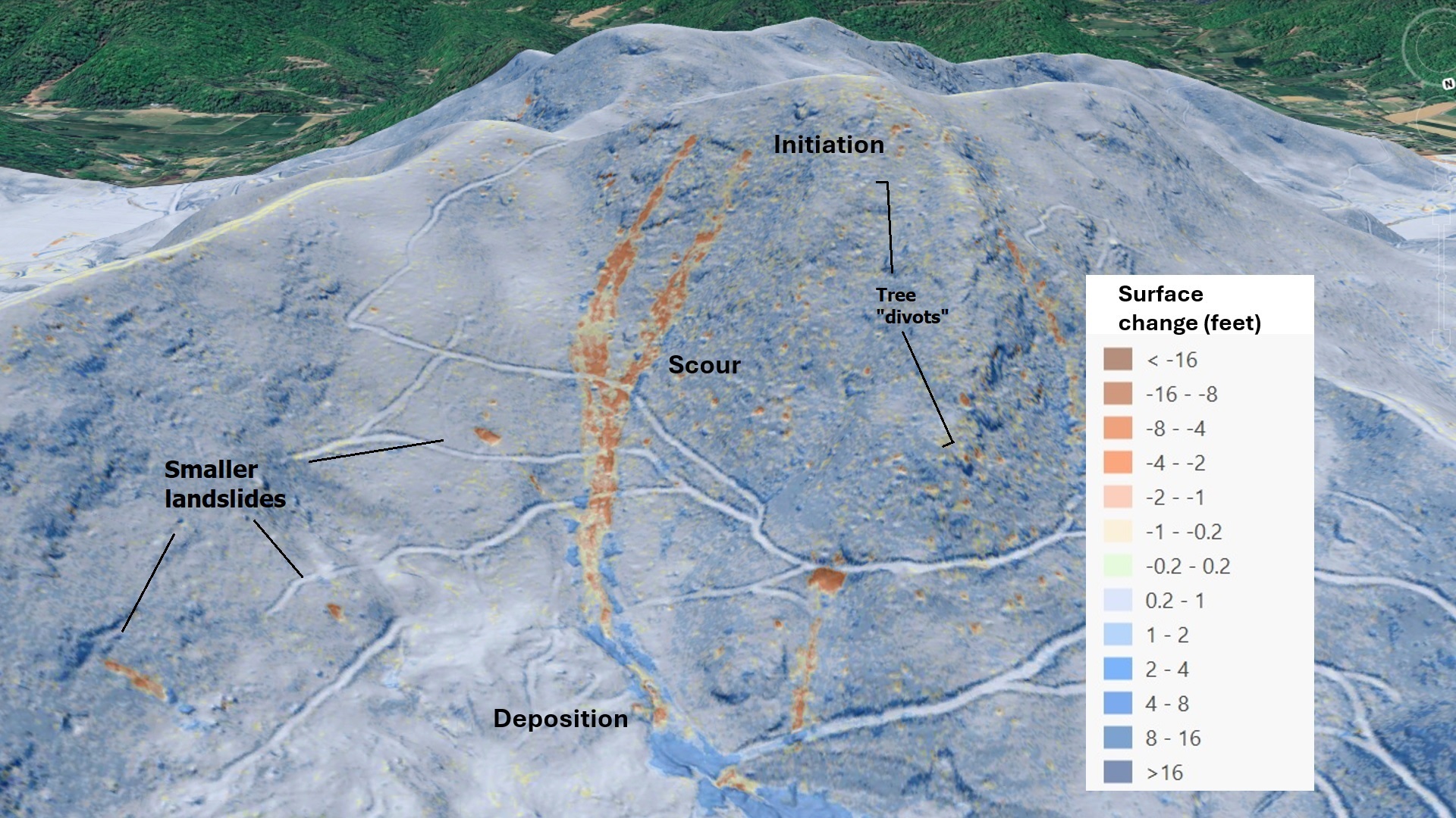
The lidar change imagery is a basic point-by-point elevation comparison from data before and after the storm. Areas lower after the storm are indicated by yellows to oranges (brown if really extreme); these are areas from which material was removed by landslide processes or water erosion. Blues highlight areas where the land is now higher from transported soil and rock debris piling up. The entire landscape is often faintly tinted due to miniscule mismatches in positioning pre- and post-data, so the combined loss (scour or down-dropping) and gain (piling up) pattern, the shape and context of identified changes, and the raw appearance of the new lidar imagery are all important for interpretation. The following GIFs give an idea of what the change patterns look like for a couple of landslide styles, starting with debris flow landslides that scour from an initiating slide and produce a deposit downslope.

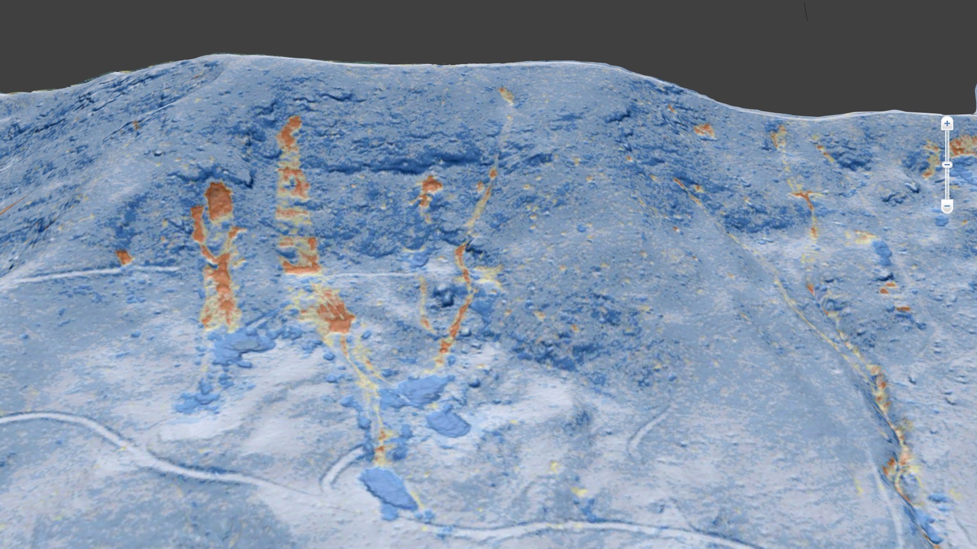
The lightest yellows indicating minor change aren’t portrayed in the diagram to keep things simple. The basic pattern is a long, red-orange track where colluvial soil is now missing from being scoured away as it fluidized within the debris flow. The scoured soil ends up in a big, blue deposit where it piled up at the bottom of the slope. This pattern is nicely visible in the first change image in the post. A tremendous number of Helene’s slides fluidized due to soil saturation but didn’t scour the slope. These “blowout” slides were incredibly numerous, and have been of great interest to ALC over years of landslide mapping because they appear to associate with the most extreme rainfall events. A blowout change pattern is illustrated in the following GIF, which also includes a scouring debris flow (image center) for comparison.
Because blowouts don’t scour the slope, they appear as closed red or orange shapes, with the colored loss area produced by the scar on the slope. Many have a blue deposit pile somewhere downslope, but others don’t, suggesting the liquefied soil spread too thin for detection or reached a channel to be transported by floodwater. Fieldwork suggests that some blowout deposit material accumulated where transported woody debris lodged on standing tree trunks and began to trap soil.
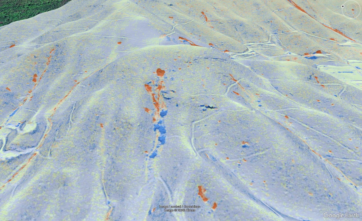
Both of the conceptual models above are well represented by the Vanderpool debris flow and surrounding slopes in Watauga County, west of Boone.
In addition to the scoured track of the debris flow and its substantial deposit, a number of small blowouts are visible. Construction changes on the lower slopes indicate work done since 2017 and are not storm-related. The yellow arrow points out a small translational slide…more on this later. While the debris flow shown here was a monster that impacted downslope properties, blowouts were the big story in Watauga County, just as they were in 1940. They dot the image of the Sugar Grove area below. A small amount of deposit appears visible well below the red scars, reflecting the extreme mobility of the fluidized soil as captured on video in the area.
Blowout-style landslides are all over the Buncombe and Watauga landscape (the only counties I have reviewed so far), and many more have been observed in other impacted counties during fieldwork. Because blowouts don’t scour a track down the slope, they can be hard to detect from aerial imagery. The following example from the headwaters of Garren Creek in Buncombe County shows how well these slides hide in the remaining forest cover. The scar is an impressive 60 feet wide. It is faintly visible in the aerial imagery once you know it’s there. This failure would have sent an impressive wave of liquefied soil, along with the few trees sitting on the failed area, downslope at high speed. No deposit, with the exception of a couple of small lumps, is visible, indicating the fluidized soil made it to the stream below (out of the frame of the image). The “vanished” material also confirms the scar’s landslide origin. No spoil is present despite the large missing volume, and no well-traveled access path (or road!) is present to mobilize machinery or personnel onto the steep slope.
Debris flows and blowouts weren’t the only slope movements triggered by Helene (remember the yellow arrow in the Vanderpool example?). Movement of intact landslide masses occurred in many locations. Due to their limited displacement, these slide movements are difficult to detect without the aid of lidar change analysis….unless one is in your backyard. Intact slides produce their own pattern of surface elevation loss and gain, with the downslope toe of the slide uplifting to various degrees as upper portions of the slide drop down along headscarps and internal scarps.
Many of these larger, slightly moving slides were reactivations of older slide features developed in huge colluvial accumulations around the flanks of steep slopes. The following images from the south side of Watch Knob, west of Swannanoa at the mouth of Bee Tree Creek, show a couple of large, intact slides. The GIF compares 2017 (pre-storm) lidar, 2025 post-storm lidar, and lidar change detection. Headscarps locations are indicated by yellow arrows; the headscarps appear as the second panel fades in. Note construction-related change at lower left, below one of the big slides.
In addition to smaller landscape details, the physical scale of the larger debris flows triggered by Helene is captured by the lidar change products. The image below shows part of the eastern prong of the Craigtown debris flow complex. The combined total length of the orange scoured tracks approaches 1.75 miles, with consistent scour depths of up to 4 feet along that entire length. Intermittent scour (with limited local deposition) continued to homes that were struck at the base of the mountain. The sheer volume of material that moved here during the three pulses over 15 minutes is staggering…and this image only shows part of it.

Lidar change imagery is also useful for understanding how landslide material moves in a storm like Helene. Some fluidized slide debris, like that from Craigtown or many of the blowouts, is incredibly mobile on both open slopes and in headwater channels. Other debris flows show less scour and mobility, despite developing from substantial initial landslides. The slide below occurred in the Big Ivy community. The upslope scar is 92 feet wide and exceeds 8 feet in depth at its center. Very limited slope erosion occurred as the initial slide debris traveled downslope, and impressive piles of deposited material developed where the landscape flattened slightly atop older, accumulated slide deposits. Whether the landscape or soil/rock characteristics reduced runout of this debris flow is unknown, but could possibly be determined through modeling and field study.
The debris flows below, from Buncombe County just west of Shope Creek, showed similarly short runouts, possibly due to topography and geology of the local ridge-forming rock from which colluvial soil is derived. The image uses the same scale change as above.
In addition to informing future modeling and hazard assessment, lidar change imagery also highlights areas that may need monitoring in future storms. The Watauga County slides at the center of the image below deposited material in a steep topographic draw, where it may be prone to saturate and fail again or be entrained by a future debris flow. Numerous examples of slide material ended up in potentially unstable locations can be identified easily, and these areas may need remediation attention.
Several geologists could devote the rest of their careers to this new lidar data and never run out of things to learn. You’ll see change results from Buncombe, Watauga, and other counties in posts on this page, and we’ll also be using them to inform fieldwork and planning in the coming months and years. As for the currently estimated 2,000 + landslides from Helene, it’s definitely on the “+” side of that…by many, many times!