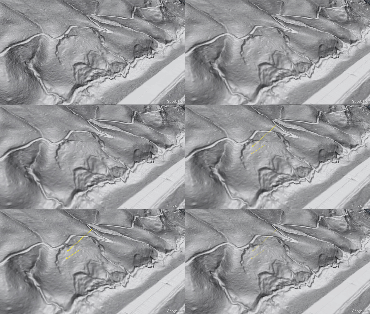
While Helene’s debris flows were the most devastating and acutely dangerous landslides of the storm, a significant number of large, slow-moving landslides were either reactivated or initiated by the extreme rainfall. This post shows two interesting reactivation examples. In both cases, erosion of an old slide toe by a flooding stream de-buttressed the slope to reactivate a dormant landslide. The movements involve large volumes of rock or soil, but are quite subtle, and might go unnoticed without LiDAR change detection. Perhaps the most impressive example, shown below, occurred along the Green River in eastern Henderson County. Look for movement of the old road grades at the center of the GIF below. The river is flowing top to bottom.

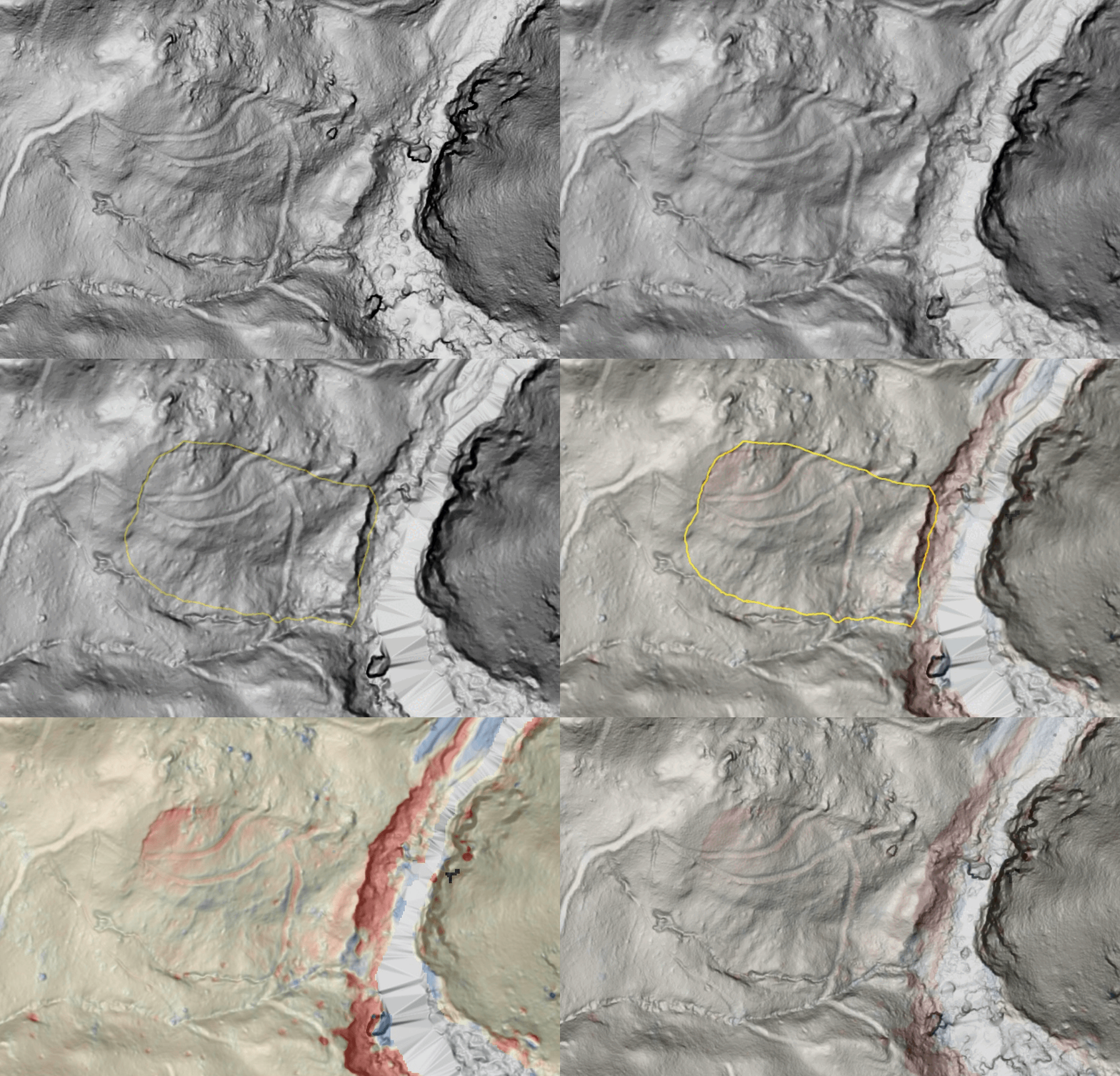
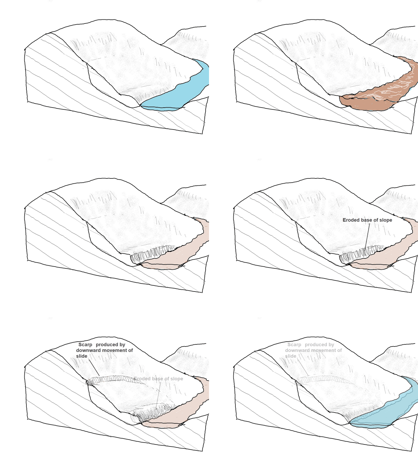
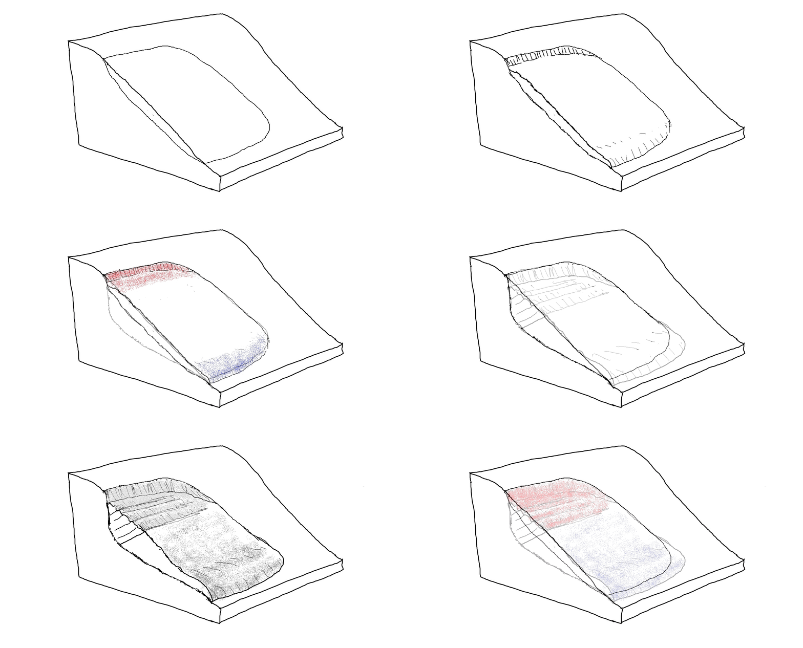
Extreme flooding of the Green River significantly eroded an existing slide toe, leading to reactivation of an area 500 ft/150 m long, 330 ft/100m wide, of unknown thickness. The movement and associated upslope scarp are visible in the GIF above when you know where to look. Red colors in the LiDAR change detection raster indicate elevation loss due to subsidence or erosional removal; blues indicate elevation gain due to bulging or deposition. While the displacement of this huge mass is low, its sheer size and connection to river erosion make it an interesting example. The GIF below provides a basic conceptual model, with exaggeration of the headscarp to make it more visible.

Seeing this slope movement at an oblique angle is useful as well, as the steepness of the topography in the area can be lost in a plan view image. The oblique view also highlights the subtlety of the movement. The shifting logging road grades provide a useful displacement reference, as does the headscarp at the upper end of the moving area.

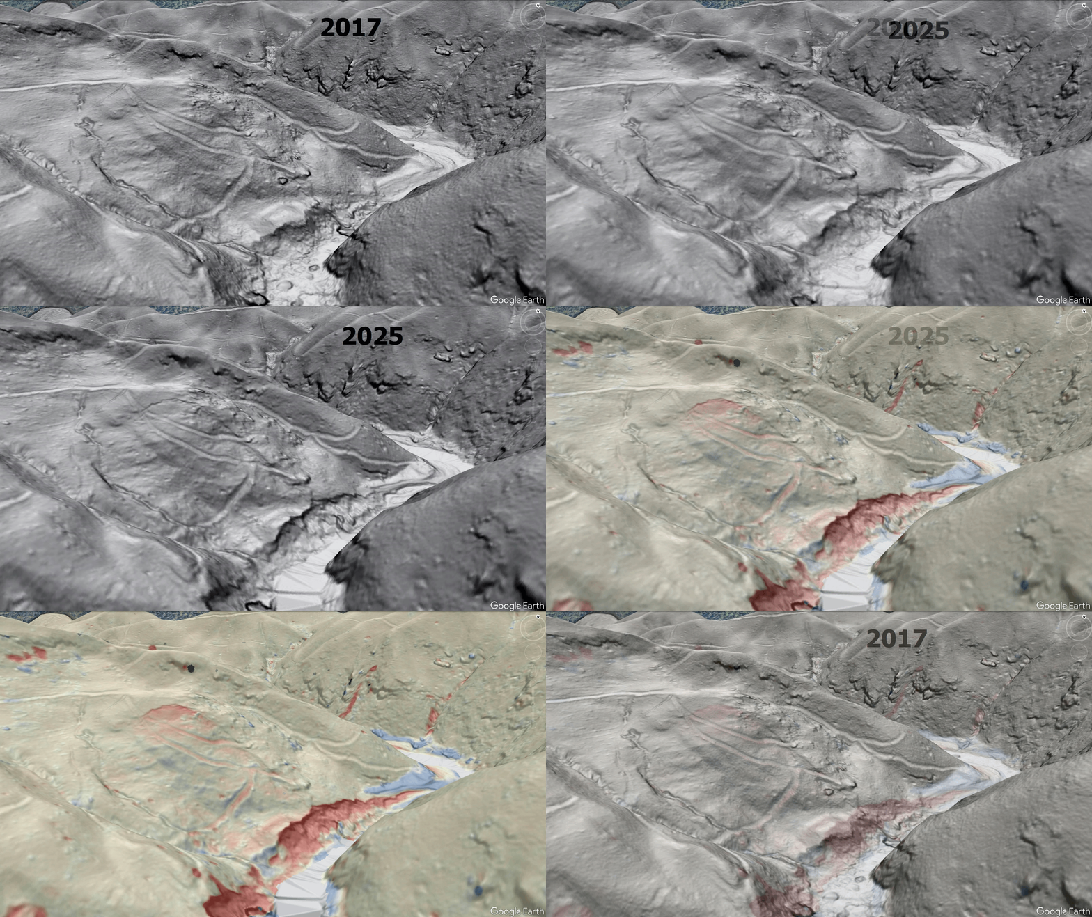
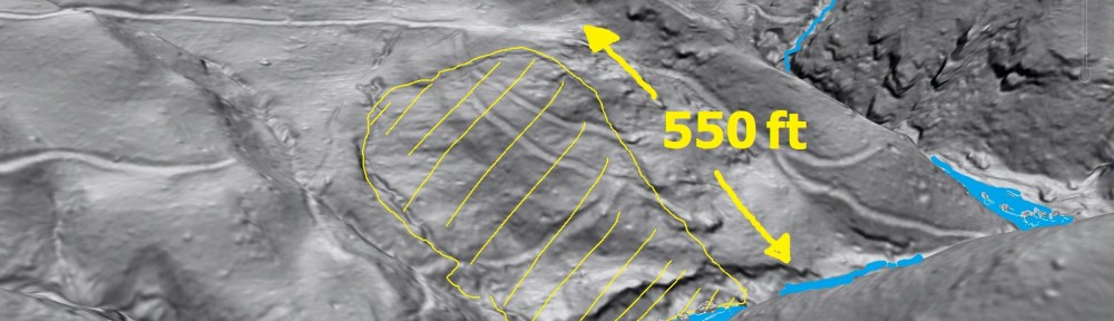
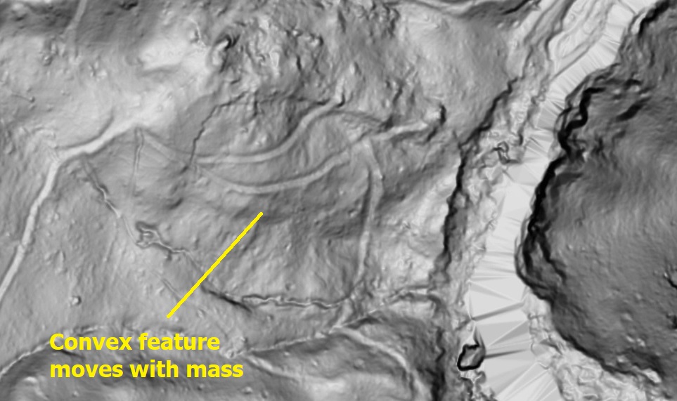
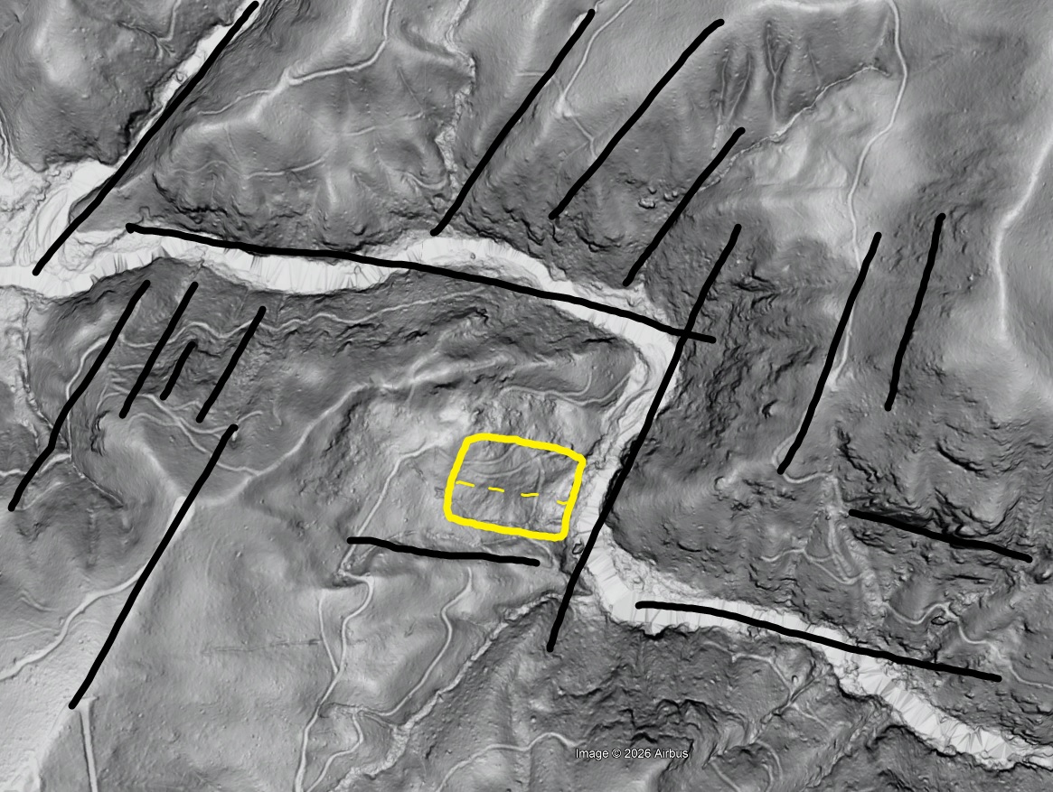
As portrayed in the conceptual diagram, this is almost certainly a reactivated rock slope movement, with the basal sliding surface occurring in bedrock as opposed to unconsolidated colluvial debris sourced from the slopes above. The lateral scarps of the sliding mass parallel bedrock structural features, as does the convex area running downslope through the middle of the slide. Movement of this convex area (dashed line; second image below), which parallels bedrock-controlled landforms at larger scale (second image below), is good evidence for a bedrock-seated slide.

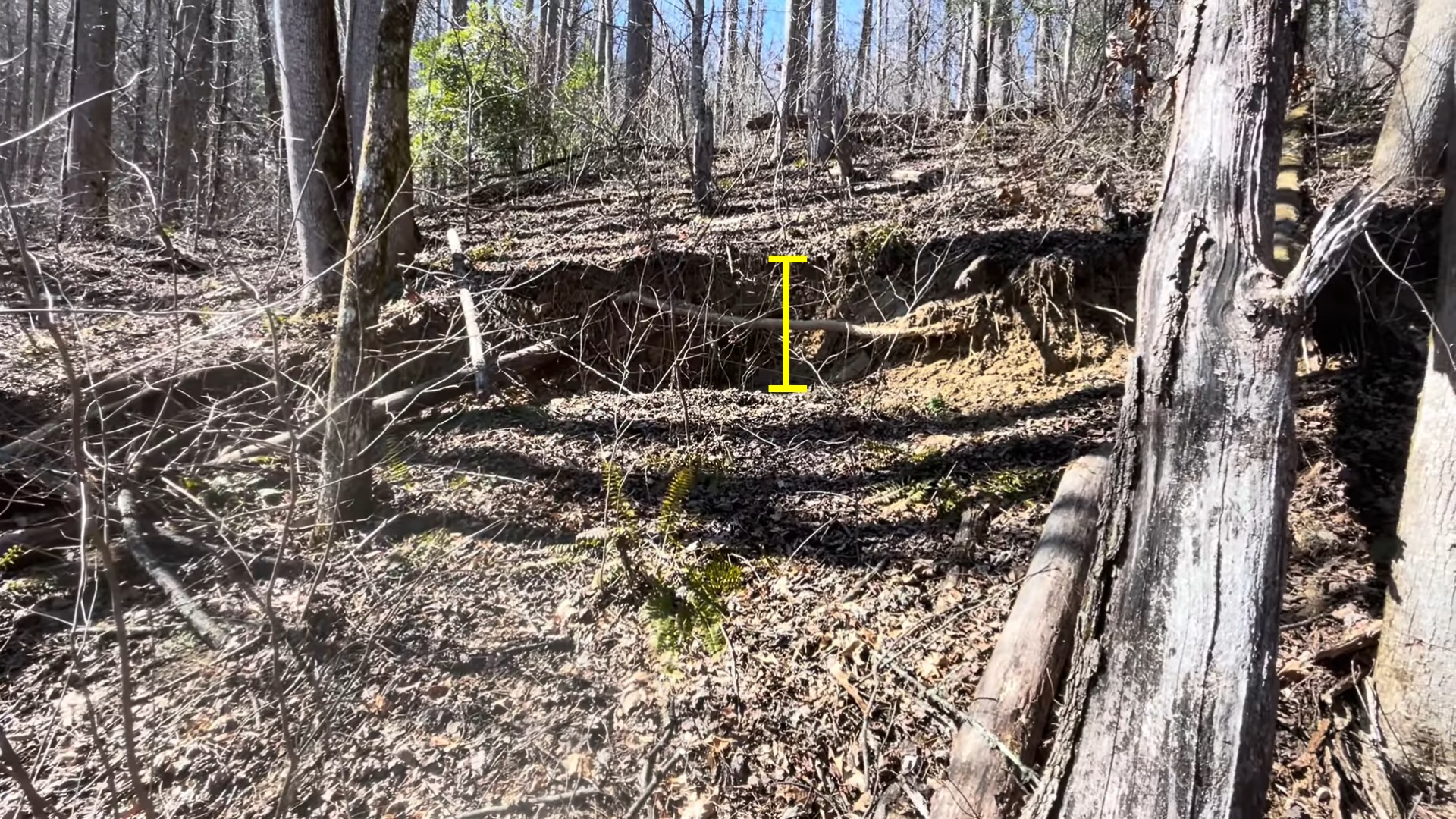
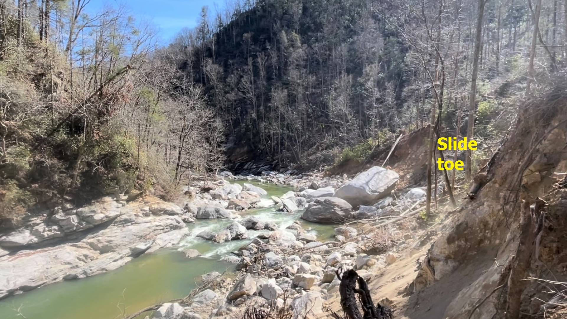
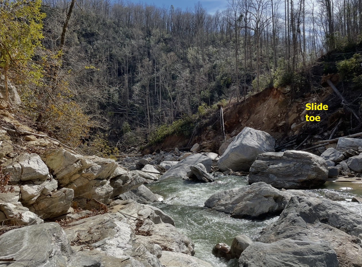
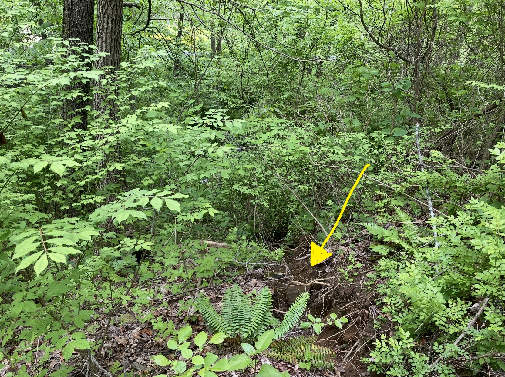
Without LiDAR imagery, we might not notice a feature like this for years, as it does not interfere with constructed features. The upper image below shows the appearance of the ~3 ft headscarp in the field. The following images show a downstream view along the slide toe, which is impressively tall. Note the bedrock ledges at left in the second and third images. These ledges indicate a generally dip slope geometry (layered structure of rock tilts downhill), suggesting a likely sliding surface.

Haywood County provides another interesting example of stream erosion reactivating a dormant slide. This example, from eastern Haywood County, involves a large debris slide, which transports colluvium (soil composed of rocky slope debris) instead of actual bedrock. The movement here is a big larger with respect to the size of the slide, which is 125 ft/37 m long and 208 ft/63 m wide. Again, thickness is unknown.

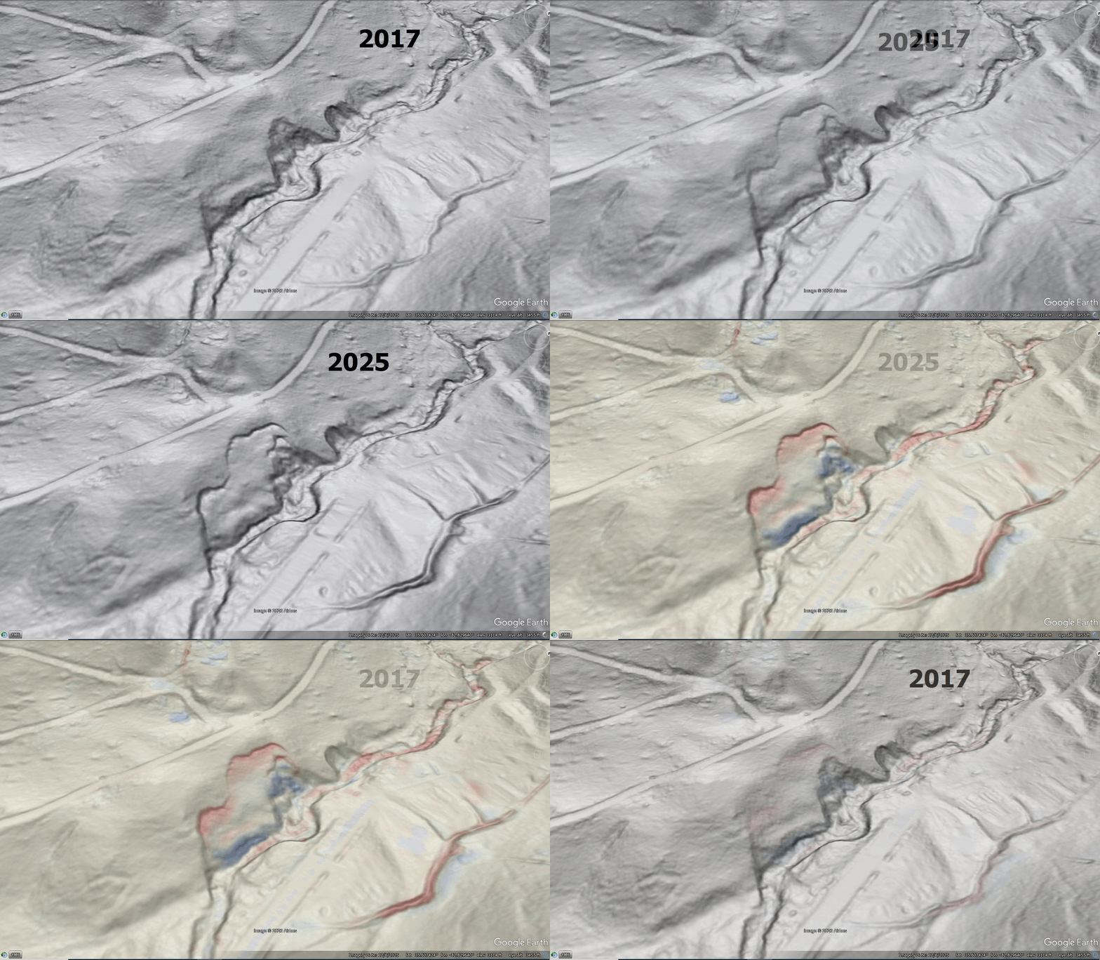
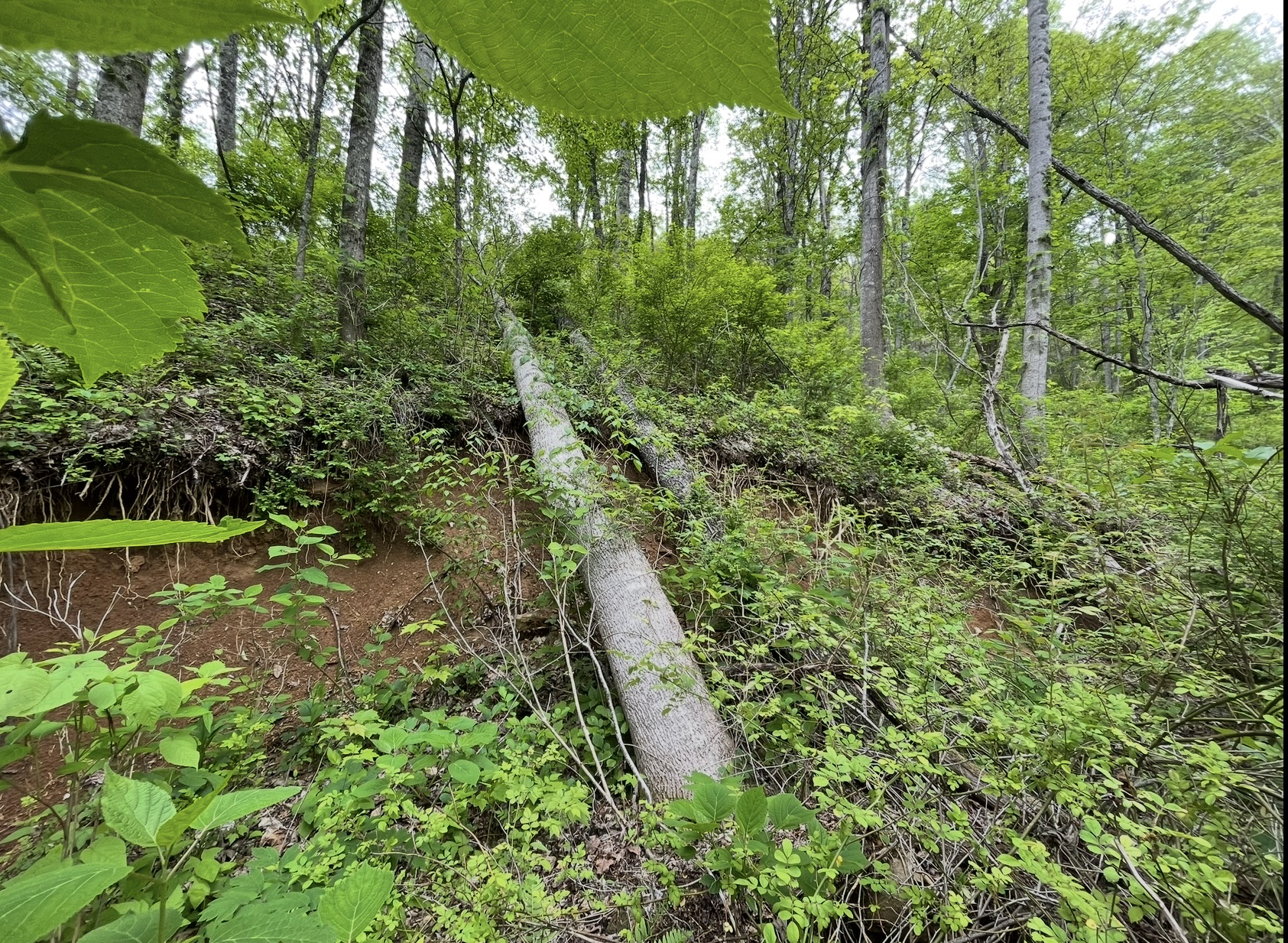
Again, red colors indicate elevation loss due to subsidence and scour, while blue indicates elevation gain due to bulging or deposition. Outside of the sliding material, this reactivated debris slide shares many characteristics with the Green River example. Toe removal de-buttressed the slope, leading to minor, but very noticeable, movement. Clearly visible scarps and tension cracks, shown below, developed at the upslope limits of the slide.

Fortunately, neither of these slides caused any damage. They are unlikely to experience significant, rapid movement, and any slight “pushing” of the stream channel is not situated to damage infrastructure or produce other spin-off effects. Were these slides to occur beneath constructed features, however, they would be a major concern and cause lots of headaches. The ability to identify this type of movement remotely, and over large areas of impacted terrain, is thus a big step forward in post-storm response.

In addition to identifying movement, the red-and-blue coloration of the LiDAR change detection imagery could, in theory, offer insight into what goes on at the base of a landslide. The GIF below provides an idealized look at this potentially useful information. A thin, translating slide undergoing little movement will produce more narrow areas of elevation loss and gain, as the shape of its sliding surface limits how the slide mass above deforms. A thicker slide, with an abrupt change in the steepness of the sliding surface, is likely to develop a wider area of elevation loss at its upslope end, accompanied by a broader area of downslope elevation gain due to outward movement of the slope.

These are idealized relationships, and roughness on the moving slope can cause confusion if, for example, an existing “hump” on the slope surface translates downhill. Even so, being able to see where, and how much, the land moved at a glance is a remarkable tool for identifying and understanding geomorphic change after a big event.

Fluidized slides (debris flows and blowouts) greatly outnumber these intact, lower displacement slides. Even so, bigger and slower features need to be identified and, in many locations, monitored, as they could potentially create impacts in the future. You’ll see more of them in future posts, for sure. Here’s one last example from just inside the South Carolina line from Henderson County, along Highway 25. Here, reactivation is visible at the slide toe and in two faint counterscarps (tips of yellow arrows) that bound a graben at the head of the slide (they’re faint, but I promise they’re there). Runoff from the road grade following the dip at the edge of the road onto the slide mass might have further encouraged its movement. The displaced area is 300 ft/90 m long and 330 ft/100 m wide.